Multivariate Functional Regression for
Classification With an Application to Geology
Vera Hofer
∗Abstract–The functional structure of data not neces-sarily requires using complex classification techniques such as support vector machines. In some appli-cations extending common multivariate methods to functional data suffices not only in regard to classifi-cation error but also and mainly to reduce time for training and testing and to keep software as sparse as possible. The present analysis demonstrates this by a classification problem in the aggregates industry. Multivariate functional regression to identify 12 dif-ferent rock types from reflectance spectra beats sup-port vector machines not only in regard to classifica-tion error but also with respect to time requirements for training and testing.
Keywords: Multivariate functional regression, sup-port vector machines, margin tree, classification, geo-engineering
1
Introduction
In many real-life applications, such as geo-engineering, signal processing, speech recognition, chemical engineer-ing, the data observed are naturally described as dis-cretized functions or curves rather than vectors of fea-ture values [26]. However, applying classic techniques of multivariate statistics directly to the functions ob-served might cause difficulties, since functions form high-dimensional and highly correlated data. This yields ill-posed problems, and in particular a substantial deterio-ration in the classification performance as well as highly imprecise parameter estimates [10] [13]. Techniques of functional data analysis can help to overcome these prob-lems of multicollinearity and diminish spurious effects.
For classification problems different approaches exist to address the functional structure of the data. First, high-dimensional classifiers such as penalized or regularized discriminant analysis [13] or support vector machines [15] [3] [14] might be applied directy to the observed data. Second, after transforming the data approprietly, com-mon classification methods might be used [27]. Most no-tably, approximating a function by a sum of basis func-tions aids further analysis. A basis expansion not only allows for representing the data as continous curves and
∗Karl-Franzens University of Graz, Department of Statistics and
Operations Research, Universitaetsstrasse 15/E3, 8010 Graz, Aus-tria, Tel: ++43-316-380-7243/ Email: [email protected]
though capturing the infinite dimension by using a few basis coefficients to represent the data, but it also yields some smoothing. Further analysis such as classification might be based on these coefficients or on scores from additional functional dimension reduction.
Third, common classification methods have been adapted to the specific structure of functional data such as linear functional discriminant analysis [13], functional logistic regression [28] [21], functional multinomial regression [1], functional penalized optimal scoring [2], a functional ver-sion of knn [10], functional support vector machines [27], or functional neural networks [30] [29] [23]. Even ensem-ble techniques that are based on the idea of constructing multiple function predictions from the data by means of a “weak” base procedure and using a convex combination of them for final aggregated prediction [6] [24] [4] [5] have been extended to functional data [11]. Basically, adapt-ing common methods to functional data makes use of the theory of Hilbert spaces. Assuming that the functions considered are from the Hilbert space L2
(R), the inner products and distances a method relys on may be re-placed by the inner product for functions and its induced metrics, respectively.
In many applications support vector machines are used for classification of functional data due to their flexibil-ity in determining nonlinear bounderies by constructing a linear boundery in a large, transformed version of the fea-ture space [14]. Yet, they avoid overfitting by controlling the margin between classes and sparsely representing the margin by the support vectors. However, disadvantes are the choice of parameters (cost, kernel and kernel parame-ters), training time, extensive memory requirements, and the problem of how to cope with multi-class problems [7] [20].
one of world’s major industries, the aggregates industry, is faced with.
The question of what extent aggregates (sand, gravel, crushed rock) resist physical and chemical loads, is of great importance for their practical use. In general, petrological composition influences engineering proper-ties of rocks such as mechanical or thermal characteristics [12] [16] [25]. Thus, a reliable method for classification of rock types and rock variants can support an appropriate choice of material [17] [18].
Due to the need for faster and more beneficial process and quality control, the aggregates industry has become inter-ested in finding automatic means for identifying suitable rock characteristics. Such a device was developed in a project called PETROSCOPE, which started in 2001 [8] [9], leading to a patent pending process [32]. Today most of the testing of aggregates is performed after production rather than at the source of the rock or sediment extrac-tion. With a more efficient test method, as promised by PETROSCOPE, it is expected that testing would in-creasingly being used for the analysis of the raw material, as well as for the end product [17] [18].
Using data from the PETROSCOPE project [19], the present investigation deals with classifying 12 different rock types or varieties of the same type with different tex-tural properties, different porosity, and different stages of alteration and surface weathering by means of their reflectance of visible and near infrared light using mul-tivariate functional regression (compare [23]). The spec-tra serve as predictors for multivariate responses that are found from class membership by a dummy variable ap-proach. Classification performance of multivariate func-tional regression, measured as classifiction error as well as time complexity, is compared to that of support vector machines.
2
Multivariate Functional Regression
2.1
Functional Regression
Let be a sample consisting of a scalar response yi and a
. In a functional regression model
yi=β0+
Z
β(t)xi(t)dt, (1)
a function β(t) and a scalar β0 ∈ R ought to be
de-termined from functional predictorsxi(t),i= 1, . . . , nto
estimate the scalaryi. Calculations simplify on
represent-ing the functions involved by basis functionsφk ∈L2(R), k = 1, . . . , K [26, p. 43]. xi(t) and β(t) need not be
represented by the same basis functions.
Letφk(t),k= 1, . . . , K be a basis for xi(t),i= 1, . . . , n
such that
xi(t) = K
X
k=1
αikφk(t) =φ ′
αi
with φ = (φ1(t), . . . , φK(t))′ and αi = (αi1, . . . , αiK)′.
Letψl(t),l= 1, . . . , Lbe a basis forβ(t) such that
β(t) =
L
X
l=1
γlψl(t) =ψ ′
γ
with ψ = (ψ1(t), . . . , ψL(t))′ and γ = (γ1, . . . , γL)′.
Thus,
Z
β(t)x(t)dt = Z
γ′ ψ φ′
αidt=
= γ′
Z
ψ φ′dt
αi=γ′
Bαi,
where B = (bij)L×K and bij = R ψi(t)φj(t)dt. Thus,
regression model (1) turns to
yi=β0+α ′ iB
′
γ. (2)
This yields classic linear regression with design matrix
X = (1 AB′
), where the ith row of Ais α′
i and 1 is a
vector of ones to account for the intercept. The solution of (2) is (β0,γ′)′= (X′X)−1X′y, wherey= (y1, . . . , yn).
2.2
Data Representation
The functions xi(t), i = 1, . . . , n, are known only for a
given set of arguments,tj∈R,j= 1, . . . , p. These
argu-ments need not be equal for all functions. Similar to [23], the observed values are assumed to bezij =xi(tj) +εij,
i.e. the function values contain some noise εij with
E(εij) = 0, i = 1, . . . , n;j = 1, . . . , p. Using a basis
representation xi(t) = K
P
k=1
αikφk(t), the functions xi(t)
can easily be determined by least squares estimation, i.e. the coefficients αik are found from minimizing
m
X
j=1 zij−
K
X
k=1
αikφk(tj)
!2
= (zi−Φαi) ′
(zi−Φαi),
where Φ = (Φjk) is a p×K matrix with Φjk =φk(tj),
zi= (zi1, . . . , zip)′. To avoid overfitting penalized
regres-sion might be carried out. For further reading cf [26, p. 86]. The estimated functions then are
xi(t) = K
X
k=1
ˆ
αikφk(t) =φ ′
ˆ
αi, (3)
where ˆαi= (Φ′Φ) −1
Φ′z
i, andφ= (φ1(t), . . . , φK(t))′.
2.3
Basis
to mirror local behaviour of the functions and not re-quire too many resources. Moreover, an easy handling is highly desirable. Wavelets are well appropriate to model local behaviour, but they are very complex and trans-forms require much time. B-splines have convenient local properties due to their finite support, but they are not orthonormal like wavelets. However, they can be calcu-lated easily and rapidly. Calculation of the basis trans-form is also less time-consuming than that of a wavelet transform. Derivatives and integrals of B-splines can eas-ily be obtained due to their polynomial structure. Thus, the spectra are represented by means of B-splines in the present analysis.
2.4
Multivariate Functional Regression
Using a basis representation, model (2) can easily be ex-tended to multivariate responses yi = (yi1, . . . , yiq) such
that
yis=β0s+
Z
βs(t)xi(t)dt=γs′Bαi,
where B andαi are defined as in section 2.1, andγs = (γs1, . . . , γsL),s= 1, . . . , q are the coefficients of the
ba-sis representation of the regression functions βs(t), i.e.
βs(t) = L
P
l=1
γslψl(t) = ψ ′
γs. The coefficients are found
from
G= (β0,Γ′
)′
= (X′
X)−1
X′
Y, (4)
where β0 = (β01, . . . , β0q)′, the design matrix is defined
as in section 2.1, andΓis anL×qmatrix whose columns areγs,s= 1, . . . , q. Yis then×qresponse matrix whose
ith row isyi= (yi1, . . . , yiq),
For classification problems the response vector is ob-tained from the vector of class labels by means of a dummy variable approach. The ith response vector yi
consists of zeros except at position s if the ith sample belongs to classs.
Several steps are necessary to estimate the class label c
of a new sample xN(t): First, the basis coefficients ˆαs
are determined by least squares estimation from the dis-cretized function zN = (zN1, . . . , zN p)′ similar to (3) by
ˆ
αN = (Φ′
Φ)−1
Φ′
zN. Second, the predictor is found from
x= (1 ˆαNn′B′), which yields ˆy=x Gusing (4). Finally,
the class label is predicted from ˆc= arg max ˆy.
3
Support Vector Machines
Support vector classification is based on finding a sep-arating hyperplane such that the margin between two groups is a maximum. In the two-group linear classi-fication problem with class labels y ∈ {−1,1}, a func-tion f(x) = β0 +β
′
x with the associated classifier
c(x) = sign[f(x)] is to be estimated fromntraining pairs
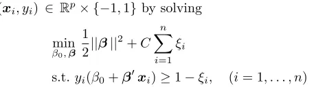
(xi, yi) ∈ Rp× {−1,1} by solving
min
β0,β
1 2||β||
2
+C n
X
i=1 ξi
s.t. yi(β0+β ′
xi)≥1−ξi, (i= 1, . . . , n)
where C is a cost parameter chosen by the user. The larger the values ofC, the higher the penalty to errors.
Different approaches exist to address the multiple class problem: margin tree support vector machines [31] or a one-against-one approach combined with majority voting [22]. Based on the marginM(i, j) = 2||β||−1
between the classesiandj, the classes are partitioned into two groups,
G1 and G2. The classifier is designed to separate these
two groups. Various ways exist to find the partition of the classes. Complete linkage clustering chooses the partition
P ={G1, G2}with the largest marginM0, i.e.
maxM(i, j)≤M0 fori, j∈Gk, k= 1,2
maxM(i, j)≥M0 fori∈G1, j∈G2
It yields more balanced trees than single linkage cluster-ing [31, p. 640].
4
Description of the Data
For 12 different rock types and varients that are of world-wide economic importance ten particles per class were se-lected and irradiated with visible and near infrared light. Depending on the sample size, 1 to 3 measurements were carried out from different postitions. Altogether, 313 spectra were collected. The measurements were made in reflectance mode from 338 nm to 1100 nm. In the present analysis only the region from 385 nm to 981 nm is consid-ered. The measurements were done with regard to control of optical geometries to attain both reproducibility and optimal inclusion of the variations of the rock surface. Table 1 gives an overview of the rock types and variants, their origin and some of their properties.
5
Results
[image:3.595.307.545.73.137.2]In the present analysis the B-spline basis for the spectra consists of 200 basis functions of order 4. The regression functions are represented by 50 B-spline basis functions of order 4. Order and number of the bases as well as the cost parameter and the kernel for support vector classifi-cation are selected by 5-fold cross-validation to minimize classification error. Thus, support vector machines use a linear kernel. Classification performance is assessed by the level of classification error and by the time required for training and testing using 5-fold cross validation and 50 runs.
Table 1: Rock type of samples and their characteristics
Rock type Place name, country code Grading [mm] Porosity Number Igneous rocks
Plutonic Rocks
Granite Ing˚a, FI 8/16 Dense 10
Gabbro Dean, GB 6/10 Dense 31
Extrusive igneous rocks (volcanics)
Rhyolite Glera, IS 8/16 Dense 10
Andesite Zagaj, SI 8/16 Dense 25
Dacite Korce, AL 8/16 Dense 36
Basalt Kloech, AT 8/16 5% 15
Sedimentary rocks
Chemical and biogenic rocks
Limestone Griza, SI 8/16 Dense 31
Dolomite Paka, SI 8/16 5% 30
Chert Mirna, SI 8/16 Dense 34
Metamorphic rocks
Amphibolite Siilinjarvi, FI 8/16 Dense 30
Gneiss Josidpol, SI 8/16 Dense 30
Serpentinite Bistrica, SI 8/16 Dense 31
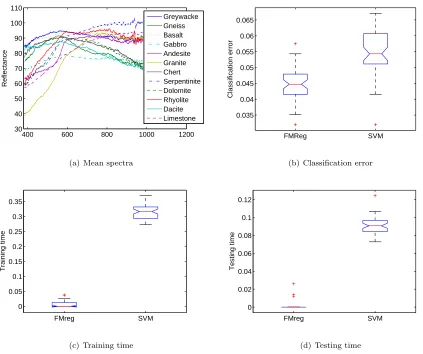
error than support verctor machines applied to the basis coefficients, which can be seen from Figure 1(b). Mean classification errors are 0.0452 and 0.0534 for multivari-ate functional regression and support vector classifica-tion, respectively. According to a sign test, classification error of multivariate functional regression is significantly smaller than of margin tree support vector machines (p-value 9.2477·10−6
[image:4.595.69.267.516.578.2]).
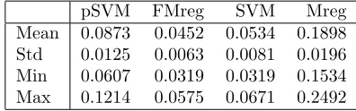
Table 2: Classification error of 50 simulation for mul-tivariate functional regression (FMreg). Pairwise SVM (pSVM), margin tree SVM (SVM) and multivariate Re-gression (Mreg) are applied to the coefficients of basis representation.
pSVM FMreg SVM Mreg
Mean 0.0873 0.0452 0.0534 0.1898
Std 0.0125 0.0063 0.0081 0.0196
Min 0.0607 0.0319 0.0319 0.1534
[image:4.595.69.271.649.724.2]Max 0.1214 0.0575 0.0671 0.2492
Table 3: Average training and testing time of 50 simu-lation for multivariate functional regression (FMreg) and margin tree SVM (SVM) applied to the coefficients of basis representation.
Training Testing
FMreg SVM FMreg SVM
Mean 0.0076 0.3154 0.0033 0.0907
Std 0.0100 0.0246 0.0063 0.0090
Min 0.0000 0.2726 0.0000 0.0728
Max 0.0377 0.3692 0.0260 0.1242
Table 2 summarizes statistics of classification error ob-tained from 50 runs of 5-fold cross validation. To show
that multivariate regression need not yield low error rates, Table 2 also gives classification error for multivari-ate regression on the coefficients of the B-spline basis rep-resentation of the spectra. Also, it shows that the worse performance of margin tree support vector machines com-pared to multivariate functional regression is not caused by the decision tree since pairwise support vector ma-chines yield even worse results.
The boxplots in Figures 1(c) and 1(d) indicate that mul-tivariate functional regression is not only much faster in training but also in testing than support vector classifi-cation, which is particularly important for time critical decision. Table 3 summarizes the statistics of training and testing time. A two-sided sign test confirms that training time (p-value 1.7764·10−15
) and testing time (p-value 1.7764·10−15
) are significantly smaller for multi-variate functional regression than for support vector ma-chines. However, it has to be mentioned that pairwise support vector machines even need significantly more time in training (p-value 0.0066) and testing (p-value 1.7764·10−15
) than margin tree support vector machines.
6
Conclusion
400 600 800 1000 1200 30
40 50 60 70 80 90 100 110
Reflectance
Greywacke Gneiss Basalt Gabbro Andesite Granite Chert Serpentinite Dolomite Rhyolite Dacite Limestone
(a) Mean spectra
FMReg SVM
0.035 0.04 0.045 0.05 0.055 0.06 0.065
Classification error
(b) Classification error
FMreg SVM
0 0.05 0.1 0.15 0.2 0.25 0.3 0.35
Training time
(c) Training time
FMreg SVM
0 0.02 0.04 0.06 0.08 0.1 0.12
Testing time
[image:5.595.83.506.76.430.2](d) Testing time
Figure 1: Mean spectra from 385 nm to 981 nm for 12 rock types.
samples cover rock types that are of worldwide economic importance and used for aggregates. Multivariate func-tional regression beats support vector machines not only in classification error but also in time requirements for training and testing. This facilitates the development of a simple and fast classification code.
7
Acknowledgements
Special thank goes to Throrgeir S. Helgason from Petro-model ehf. in Reykjavik, Iceland for his idea to analyse aggregates statistically, for lauching the EUREKA PET-ROSCOPE project and for managing sampling and pro-viding the data. Thanks also goes to Ana Mladenovic at ZAG Ljubljana, Andrew Nevitt at RMC Materials Ltd (now CEMEX UK Operations Ltd), Hanna J¨arvenp¨a¨a Lohja Rudus Oy, FI, Karsten Iversen at Linuhoennun hf, Iceland, for time consuming sampling and analyses of the samples. Finally, thank goes to John Knight at Knight Photonics Ltd., UK, for his useful comments at the final stage of the work.
References
[1] Aguilera A., Escabias M., Solving Multicollinearity in Functional Multinomial Logit Models for Nomi-nal and OrdiNomi-nal Respones, in: Dabo-Niang S., Fer-raty F. (eds), Functional and Operational Statistics, 2008, pp. 7 –13
[2] Ando T., Penalized optiaml scoring for the classifica-tion of multi-dimensional funcclassifica-tional data, Statistical Methodology, V6, pp. 565 – 576, 2009
[3] Cristianini N., Shawe-Taylor J., 2004. An Introduc-tion to Support Vector Machines: Cambridge Uni-versity Press.
[4] Breiman, L., 1998. Arcing classifiers. Annals of Statistics 26, 801–824
[5] Breiman, L., 1999. Prediction games and arcing al-gorithms. Neural Computation 11, 1493–1517
[7] Burges C.J.C., A tutorial on support vector ma-chines for pattern recognition, Data Mining and Knowledge Discovery, V2, N2, pp. 121167, 1998
[8] EUREKA 2001, PETROSCOPE – An Optical Anal-yser for Construction Aggregates and Rocks, Project no. 2569, Announced 28 June 2001, EUREKA, Brus-sels.
[9] EUREKA, 2005, PETROSCOPE II – An Optical Analyser for Construction Aggregates and Rocks, Project no. 3665, Announced 01 June 2005, EU-REKA, Brussels.
[10] Ferraty, F., Vieu, P., “Curve Discrimination. A Non-parametric Functional Approach“, Computational Statistics & Data AnalysisV44, pp. 161–173, 2003
[11] Ferraty, F., Vieu, P., “Additive prediction and boosting for functional data“,Computational Statis-tics & Data AnalysisV44, pp. 1400 – 1413, 2009
[12] Griffiths J.C., 1967, Scientific method in analysis of sediments: McGraw-Hill, New York, 508 pp.
[13] Hastie T.J., Tibshirani R.J., Buja A., 1995. Penal-ized Discriminant Analysis, Annals of Statistics, v. 23, p. 73 –102.
[14] Hastie T.J., Tibshirani R.J., Friedman J., 2001. The Elements of Statistical Learning, Data Mining, In-ference and Prediction, Springer New York, Berlin, Heidelberg.
[15] Hastie, T.J., Rosset, S., Tibshirani, R., and Zhu, J., 2004, The Entire Regularization Path for the Sup-port Vector Machine: Journal of Machine Learning Research v. 5, p. 1391 – 1415.
[16] Helgason, Th. S., 1990, Characteristics, properties, and quality rating of Icelandic volcanic aggregates: 43rd Canadian Geotechnical Conference, St. Foy, Universit´e Laval, 1, p. 339–345.
[17] Hofer V., Pilz J., Helgason T.S., 2006, Statistical Classification of Different Petrographic Varieties of Aggregates by Means of Near and Mid Infrared Spec-tra: Mathematical Geology 38 (7), 851 – 870.
[18] Hofer, V., Pilz, J., and Helgason, T.S., 2007, Sup-port Vector Machines for Classification of Aggre-gates by Means of IR-Spectra: Mathematical Ge-ology 39 (3), p. 307 – 319.
[19] Hofer, V., Pilz, J., and Helgason, T.S., 2010, Func-tional Margin Tree Classification of Different Pet-rographic Varieties of Aggregates by Means of Re-flectance Spectra, Mathematical Geosciences, (ac-cepted for 2010)
[20] Horv´ath G., Neural networks in measurement sys-tems (an engineering view), in: Suykens J. et al. (eds.), Advances in learning theory: methods, mod-els, and applications, Series 3: Computer and Sys-tems Sciences, NATO Science Series, V190, 375 – 396, 2003
[21] James, G.M., Generalized linear models with func-tional predictors, Journal of the Royal Statistical So-ciety, V64, P3, pp. 411 – 432, 2002
[22] Hsu C.-W., Lin C.-J., 2002, A Comparison of Meth-ods for Multi-Class Support Vector Machines, IEEE Transactions on Neural Networks, v. 13, no. 2, p. 415 – 425.
[23] L´opez M., Mart´ınez J., Mat´ıas J.M., Taboada J., Vil´an J., Functional classification of ornamental stone using machine learning techniques, Journal of Computational and Applied Mathematics, 2010, doi:10.1016/j.cam.2010.01.054
[24] Lutz R.W., Buehlmann, P., 2006. Boosting for high-multivariate responses in high-dimensional linear re-gression,Statistica Sinica 16, 471–494.
[25] Mitchell, J.K., 1993, Fundamentals of soil behavior: 2nd edition, Wiley, New York, 437 pp.
[26] Ramsay, J.O., and Silverman, B.W., 2005, Func-tional Data Analysis, 2nd ed., Springer Series in Statistics, New York, 426 pp.
[27] Rossi, F., Villa, N., 2006, Support vector machines for functional data classification, Neurocomputing, v. 69, 730 – 742.
[28] Rossi N., Wang X., Ramsay J.O.Nonparametric Item Response Function Estimates with the EM algorithm, Journal of Educational and Behavioral Statistics, V27, pp. 291 – 317, 2002
[29] Rossi F., Conan-Guez B., Functional multi-layer perceptron: a non-linear tool for functional data analysis, Neural Networks, V18, 45 – 60, 2005
[30] Rossi F., Delannayc N., Conan-Gueza B., Verleysenc M., Representation of functional data in neural net-works, Neurocomputing, V64, pp. 183 – 210, 2005
[31] Tibshirani R., Hastie T., Margin trees for high-dimensional classification, 2007, Journal of Machine Learning Research v. 8, p. 637 – 652.