Data mining approaches for detecting intrusion using UNIX process execution traces

1-1-2000

Data mining approaches for detecting intrusion

using UNIX process execution traces

Xiaoning Xiaoning

Follow this and additional works at:https://lib.dr.iastate.edu/rtd Part of theBusiness Commons

This Thesis is brought to you for free and open access by the Iowa State University Capstones, Theses and Dissertations at Iowa State University Digital Repository. It has been accepted for inclusion in Retrospective Theses and Dissertations by an authorized administrator of Iowa State University Digital Repository. For more information, please [email protected].

Recommended Citation

Xiaoning, Xiaoning, "Data mining approaches for detecting intrusion using UNIX process execution traces" (2000).Retrospective Theses and Dissertations. 17791.

by

Xiaoning Zhang

A thesis submitted to the graduate faculty

in partial fulfillment of the requirements for the degree of MASTER OF SCIENCE

Major: Business Major Professor: Dan Zhu

Iowa State University Ames, Iowa

Graduate College Iowa State University

This is to certify that the Master's thesis of Xiaoning Zhang

has met the thesis requirements of Iowa State University

TABLE OF CONTENTS

CHAPTER 1 INTRODUCTION 1.1 Overview

1.2 Purpose of the Study 1.3 Structure of the Thesis

CHAPTER 2 LITERATURE REVIEW 2.1 IDS Analysis Approaches

2.1.1 Misuse Detection 2.1.2 Anomaly Detection

2.2 Strategies for Data Collection and Analysis 2.2.1 Keyboard Level

2.2.2 Low Level System Calls 2.2.3 Command Level

2.2.4 Application Level

2.3 Methods to Analyze System Calls 2.3.1 TIDE and STIDE

2.3.2 Machine Leaming Approach 2.4 Summary

CHAPTER 3 METHODOLOGY

3.1 Neural Networks and Backpropagation Net 3 .1.1 Overview

3.1.2 Backpropagation Net 3.2 Rule Induction: ID3 and C4.5

3.2.1 Overview 3.2.2 C4.5 3.3 Rough Sets

3.3.1 Overview 3.3.2 Basic Concept

3.3.3 Advantages of Rough Sets 3.4 Summary

CHAPTER 4 COMPARISON OF PERFORMANCES OF THREE METHODS

4.1 Preparation and Experiment 4.1.1 Data Description 4.1.2 Data Preparation

4.1.3 Training and Testing Data Representation 4.1.4 BP Experiment

4.1.5 C4.5 Experiment 4.1.6 Rough Sets Experiment 4.2 Result and Discussion

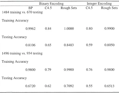
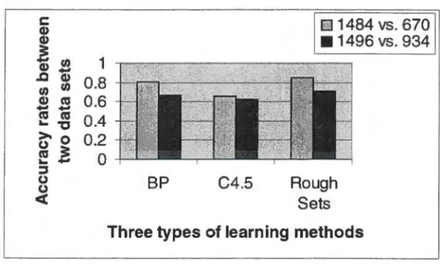
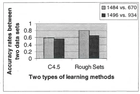
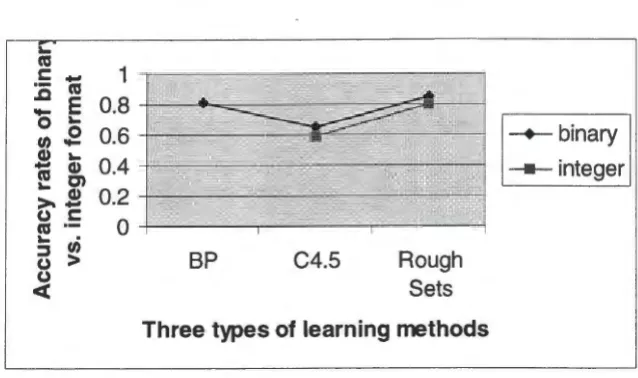
4.2.1 Accuracy Rates vs. Data Combinations 4.2.2 Accuracy Rates vs. Data Representations 4.2.3 Overall Prediction Performance

4.2.4 True Positive and False Positive 4.3 Summary

CHAPTER 5 CONCLUSIONS 5.1 Summary

5.2 Contribution

5.3 Directions of Future Works APPENDIX

REFERENCES

ACKNOWLEDGMENTS

INTRODUCTION

In this chapter, we give a broad overview of the field of network security and the motivation for employing various techniques to automate audit data analysis in the intrusion detection systems. In the following chapters, we will survey the intrusion detection methods in detail.

1.1 Overview

During the past few years, information technology has become a key component to support the critical infrastructure of the world. The public telephone network, banking and finance, vital human services, and other critical infrastructures are dependent upon information technology for their day-to-day operation. Every day, millions of people use computers to process or search for different kinds of information. While most of these users access data legitimately, some use illicit ways to access computers. Thus, computer security becomes a major concern among various industries, especially those organizations depending heavily on networks.

growing emphasis on the Internet are causing organizations to feel more and more insecure about their networks. These three trends result in significantly higher exposure to both internal and external attacks. Some of the attacks come from the inside the organization because of misuse within the system, while many attacks are carried out by outside hackers. According to a leading survey, the number of computer security breaches has risen 22% between 1996 to 1998, with $136 million associated losses. The U.S. General Accounting Office (GAO) disclosed that approximately 250,000 break-ins into Federal computer systems were attempted during the year of 1996 and 64% of these attacks were successful. Worse yet, the number of attacks is doubling every year. Based on previous studies, the GAO estimates that only 1- 4% of these attacks will be detected and only about 1 % will be reported (Durst et al., 1999). In the beginning of February 2000, several major web sites including Yahoo, Amazon, eBay, Datek, and eTrade were shut down because of the denial-of-service attacks created on their web servers.

Since computer systems are increasingly vulnerable to attack, the network security is an important issue for most organizations. A variety of security devices and actions are being deployed to secure networks. There are mainly two types of techniques: protection and detection.

Protection techniques are designed to guard hardware, software and user data against threats from both outsiders as well as from malicious insiders. One type of security device receiving considerable amount of attention is the firewall. A firewall interposes a barrier at

require the accurate configuration of numerous and confusing access control lists. These configurations must be continually updated to allow access to new network services and to keep up with changing security policies. Even properly configured firewalls have known weak spots. In many situations, hackers can circumvent firewalls entirely and enter the system without being noticed. Another disadvantage is that firewalls cannot prevent attacks from the inside the network, which is also a frequent source of break-ins.

In addition to firewalls, encryption and operating system access controls also provide protective functions. Operating systems provide user authentication through passwords and multi-level access control to information. Encryption techniques can hide the true information by converting it into an unrecognized format. Regardless of these strong protection measures, people cannot be completely successful in preventing problems. Hackers continually find new ways to break into or interfere with systems. Moreover, most mechanisms are powerless against misbehavior by legitimate users who perform an authorized actions.

Intrusion detection systems (IDS) and vulnerability assessment systems (also known as scanners) are a good complement of protective tools for network security. Organizations have eagerly adopted detective products in the last several years. In a report by the Internet Security Systems Inc, they have supplied more than 10,000 detection engines for companies and government sites. According to industry estimates, the market for intrusion detection products has grown from $40 million in 1997 to $100 million in 1998.

problematic settings, system password files for weak passwords, and other system objects for security policy violations. Although these systems cannot reliably detect an attack in progress, they can determine the possible weak points for attack.

IDS help computer systems prepare for and deal with attacks. They collect information from a variety of systems and network sources, then analyze the information for signs of intrusion and misuse. The majority of functions performed by IDS include:

• monitoring and analyzing user and system activity, • assessing the integrity of critical system and data files, • recognizing activity patterns reflecting known attacks, • responding automatically to detected activity, and • reporting the outcome of the detection process.

The success of an intrusion detection system can be characterized by both false alarm rates and detection efficiency (Stillerman et al., 1999). Since the audit services record the occurrence of all security-relevant events, which result in an enormous quantity of audit data, using the correct method to analyze the proper set of system data becomes an important issue to keep false alarm rates to low level and have high detection efficiency.

1.2 Purpose of the Study

The data we used comes from the web site of the computer immune system, a network

security research project conducted by Professor Forrest at the University of New Mexico

and her students. They and another research group at Columbia University (Lee and Stolfo,

1997, 1998) analyzed this set of data using different techniques. In our experiment, we used

a binary representation method different from those in their studies, and tried to determine

whether C4.5, Rough Sets and Backpropagation net can discover the patterns behind the

sequence-related data as efficiently as their methods.

1.3 Structure of the Thesis

This thesis includes five parts. Following this introduction, there is a comprehensive

survey of existing intrusion detection methods; the third chapter is a review of the main

methodologies utilized in our experiment including C4.5, Backpropagation net and Rough

Sets. The fourth chapter explains in detail the experiment and results for the comparison

between the three methodologies. The last chapter presents the conclusions of our

CHAPTER2 LITERATURE REVIEW

In this chapter, first we will have a thorough discussion about the intrusion detection system, especially the analysis methods and their advantages and disadvantages. Then, we will give an overview of the analysis data used in IDS and focus on research of the system

calls.

2.1 IDS Analysis Approaches

IDS can be generally divided into two categories according to the analysis method. These categories are misuse detection system and anomaly detection system. Misuse detection system detects attacks based on well-known vulnerabilities and intrusions stored in a database, while anomaly detection system detects deviation of activity from normal

profiles.

2.1.1 Misuse Detection

Misuse detection is signature-based detection. When the intrusion signatures are matched by new audit data, the detector flags intrusions and sets off an alarm.

The techniques used for misuse detection are expert systems, model-based reasoning

systems, state transition analysis, genetic algorithm, fuzzy logic, and keystroke monitoring.

The discussions of various misuse detection approaches are in the following.

2.1.1.1 Expert Systems

Human experts encode the knowledge about vulnerabilities and past intrusions in

"if-then" rules. Conditions causing intrusions are specified in the "if' part, and reactions to the

relative attacks are encoded in the "then" part. When all these conditions are satisfied, the

actions corresponding to them occur. Examples using this implementation are described in

various studies (Snapp and Smaha, 1992; Porras and Valdes, 1998). In the EMERALD

system developed by SRI International (Porras and Valdes, 1998), signature engines are used

to analyze an event stream. If the stream is mapped to an abstract representation of abnormal

event sequences, it indicates danger to the system. The signature engine is essentially an

expert system whose rules indicate suspicious activities.

2.1.1.2 State Transition Analysis

State Transition Analysis Tool (ST AT) is a method in which penetration is viewed as a

sequence of actions that make the system from the initial state prior to an attack to the final

compromised state after the attack occurs (Porras, 1992). The system converts penetration

scenarios into state transition diagrams, which are special rules representing dangerous

activities. States in the attack pattern correspond to system states and have boolean

assertions associated with them that must be satisfied to transit to that state. Successive

2.1.1.3 Keystroke Monitoring

This technique utilizes user keystrokes to determine the occurrence of an attack.

Primarily, there should be a pattern match for specific keystroke sequences that indicate an

attack. The disadvantage of this approach is the lack of reliable mechanisms for user

keystroke capture without the operating system support.

2.1.1.4 Model-Based Reasoning Intrusion Detection

In this approach, a database of attack scenarios is specified in terms of sequence of user

behavior (Garvey and Lunt, 1991). The system would reason about hypothesized intrusions

by gathering evidence from audit trails and statistical profiles, and determining the likelihood

of specific hypothesized intrusion scenarios. If one model of intrusion is discovered, the

system continues to predict the steps expected to occur in the intrusion scenario, until enough

evidence is above a threshold value confirms the intrusion.

2.1.1.5 Genetic Algorithms

Genetic algorithms, proposed by Holland (1975), are optimum search algorithms based

on the mechanism of natural selection in a population. The potential solutions to the problem

are represented in strings. The population is randomly initialized; in every generation,

mutation and crossover are applied to the strings to obtain new strings; then a set of fittest

solution is chosen from the combined population for the next generation. The fitness of each

individual is simply the value of the function to be optimized (the fitness function).

Ludovic

Me (

a genetic algorithm. The goal was to determine, among all the possible attack subsets and

system. They represented a string in an Na length of individuals with values of 1 or 0, where

NO is the number of potential attacks. The fitness function is given as:

Nu

Fitness= a+ (

LWJ; -

fJJ'} ),

where I is an individual, W; is the weight associated with the attack i, and

/Jf',2 is a penalty

function. The ~ parameter makes it possible to modify the slope of the penalty function, and

a sets a threshold to create a positive fitness function making the fitness positive. The three

basic operators they used were proportionate selection, one-point crossover, and simple mutation.

2.1.1.6 Time-Based Inductively Machine (TIM)

This approach was proposed by Teng et al. (1990). The main difference between TIM

and other rule-based detection systems is that TIM focuses on patterns of event sequences,

whereas the others focus on individual events. It is an approach using a time-based inductive engine to generate rule-based symbolic sequential patterns from observations of a temporal

process. These patterns are used to predict the next possible events with satisfactory accuracy. When the subsequent events deviate significantly from the established patterns, it will be considered a violation of their rules, indicating the possibility of an intrusion.

2.1.1.7 Fuzzy Logic

RETISS is a real time security system for threat detection developed by F. Carrettoni et

al. (1991). It is based on the assumption that there exists a correlation between anomalous user behavior and threats. There are security rules to be enforced to express this correlation.

and object involved are defined in a weight table for each rule. The weight table is a

7-column table with the form

< Subj_class, Obj_class, Action, Anomaly, Occurrence, Weight, Threshold>.

These levels are combined using fuzzy logic to express the probability of a given threat.

There are several components in this system: the Audit Record File (ADF), the Data Base

(DB), the Knowledge Base (KB), the Audit Record Analyzer (ARA), the Threat Detection

Module (TDM), the Profile Updating Module (PUM), and the Interface Module (IM).

Among them, ARA, TDM, and KB are the key components enforcing the detection control.

ARA is used to examine the ADF to evaluate if there are audit records corresponding to

suspicious actions in the KB. Upon reception of an anomaly record by the ARA, the TDM

checks the KB, firing every rule with a trigger matching the anomaly record under

consideration. When a rule is fired, its antecedent is evaluated. If the antecedent is not

satisfied, then no threat is pointed out, otherwise the system must evaluate how dangerous the

threat is. Evaluation of the level of danger of anomalous behavior is enforced using the

weight table associated to the rule. Tuple's weight is multiplied by the user_weight of the

user specified in the anomaly record under consideration to get the evaluation_

record_ weight. All these values are combined replacing AND/OR operators in the rule

antecedent. The result is a numerical value expressing the level of danger of a given threat.

If the value is greater than the specified threshold, then an alarm is generated.

2.1.1.8 Summary of Misuse Approach

One advantage of misuse detection is that it allows sensors to collect a more tightly

targeted set of system data, thereby reducing the system overhead. It also has some

knowledge of attacks. Since there are attacks which have never been tried, or vulnerabilities yet to be discovered, we cannot always make a complete list of rules for the detection system. Furthermore, not every attack can be perfectly represented by the "expert system" or some kinds of rules. If an intrusion scenario does not trigger a rule or triggers an incomplete rule, it will not be detected by this rule-based approach. Last, because new attacks or new versions of attacks appear continuously to replace those old scenarios, the complexity of the databases grows as the number of well-known attacks grows, introducing problems of scale. It is difficult to keep them updated as the catalog of attacks grows.

2.1.2 Anomaly Detection

The goal of the anomaly detection system is to recognize behaviors that deviate from normal activities. In different anomaly detection approaches, the normal profiles include various kinds of measuring variables of the system objects, and they are represented in different styles. However, the basic working theory is to compare the observed activities with the normal profiles and find the deviations. There are always some thresholds to specify for the detection system. If the deviation is higher than the threshold, the computer system will be considered to be attacked, otherwise, the deviation will be neglected. The challenge is to define the threshold in a way that minimizes the false alarm rate and maximizes the detection efficiency.

2.1.2.1 Statistical Approach

Statistical profiles are created for system objects (e.g., users, files, directories, devices, etc.) by measuring various attributes of normal use (e.g., number of accesses, number of times an operation fails, time of day, etc.). Mean frequencies and measures of variability are

values fall outside the normal range. For example, statistical analysis might signal an unusual event if an accountant who had never previously logged into the network outside the hours of 8 AM to 6 PM were to access the system at 2 AM.

NIDES (Lunt et al. 1992) is an example of a statistical approach. The anomaly detector observes the activity of subjects and generates profiles for them to represent their behaviors.

There are several types of measures (M 1 , M 2 , M 3 , .•. , Mn ) comprising a normal profile,

every measure has a value (S 1 , S 2 , S 3 , ••• , Sn ) presenting the abnormality of the profile. A

higher value of S; indicates a greater abnormality. A combining function of the individual S

values may be the weighted sum of its squares, as in

where a; reflects the weight of the metric M.

In the previous part of this chapter, there was an introduction of the expert system of EMERALD (Porras and Valdes 1998). This system also includes a statistical analysis tool.

There are four classes of measures employed by statistical algorithms--categorical,

continuous, intensity, and event distribution. The system maintains a description of a subject's behavior in a profile subdivided into short- and term elements. The long-term profile is adapted to changes in subject activity slowly, while the short- long-term profile represents recent activities and accumulates values between updates. The differences between short- and long- term profiles is compared to a historically adaptive, subject-specific

The advantage of the statistical approach is that statistics has been well studied. It

provides us with a complete theory base for research. However, there does exist some

disadvantages. First, it is insensitive to the order of occurrence of events, which will miss an

important measure for intrusion detection. Second, intruders can gradually train it so that a

behavior once regarded as abnormal will be normal after intended training. Also, it is

difficult to decide the threshold beyond which there will be an intrusion considered.

2.1.2.2 TIDE and STIDE

Hofmeyr et al. (1998, 1997) and Forrest et al. (1996) at the University of New Mexico

developed these two methods, time-delay embedding (TIDE) and sequence time-delay

embedding (STIDE). They used lookahead pairs or fixed length sequences of system calls to

set up the normal profile, compared them with certain process traces, and utilized some

statistical indexes, such as local frame frequency and Hamming Distance to analyze the

comparison results. We will discuss this method in detail later in this chapter.

2.1.2.3 Neural Networks

There are several neural network algorithms employed in intrusion detection research.

Bonifacio et al. ( 1997) and Herve DeBar et al. (1992) used Backpropagation, QuickProp and

Rprop. Kohonen's self-organizing feature map was used by Fox et al. (1990).

The basic idea of these methods is to train the neural net with both normal and abnormal

system features at first. The weights of each neuron (or node) are adjusted in the process of

training. When it is used in the real detection system, it can classify the audit data into

• The success of this approach does not depend on any statistical assumptions about the

nature of the underlying data.

• Neural nets cope well with noisy data.

• Neural nets can automatically account for correlation between the various measures

that affect the output.

On the other hand, training a neural net is a time-consuming task. Parameters of the

neural network topology and learning are determined only after considerable trial and error.

Another disadvantage is that although the neural networks get a satisfied result, it is still hard

to determine theory explanations about the results.

2.1.2.4 Machine Learning Approach

Rule induction technique is widely used in the classification, pattern recognition, and

optimization problems. Lee and Stolfo (1997) used RIPPER (Cohen 1995), a rule learning

method, to learn the normal and/or abnormal patterns from certain audit system features.

Since they used the same set of data employed in our experiment, we will discuss their

experiment in detail later in this chapter.

2.1.2.5 Immune System

Forrest et al. (1996, 1993) proposed an artificial immune system simulating the human

immunology system to detect intrusions. Kim and Bentley (1999a, b, c) proposed a negative

selection algorithm based on Forrest et al.' s immune system. Their primary theory is that a

computer security system should protect itself from unauthorized intruders, which is similar

to the human immune system protecting the body (self) from invasion by inimical microbes

connection into a single 49-bit binary string. Self is a set of normal occurring connections,

while non-self is a set of connections not normally observed on the networks.

There are three learning mechanisms used by immune system. Negative selection is the

first step, which means randomly created detectors (also 49-bit strings) would be killed when

they match any one string in the "self." After this period, survived detectors become mature.

The second step is maturation of na"ive cells into memory cells. During some period after

detector becomes mature, there will be new connection matches its pattern. If there are a

sufficient number of packets detected (in another words, they match some patterns of the

mature detectors), an alarm will be raised. But if a detector failed to match any connections,

it will be killed too for its uselessness. This step can compress the detectors into a minimized

set in order to save the system resource and speed up the detection process. The third step is

some kind of genetic algorithm method called "affinity maturation." Since it is possible all

redundant detectors to similar intrusions survived in a single "self' set, there will be a waste

of system resource. So, the immune system is designed to make detectors compete against

each other, the ones with the closest match (greatest fitness) will win and survive at last.

After these three steps, an efficient "self' detector set will be created and can be used to

detect intrusion in the future. Since detectors can be randomly created continuously, this

"self' set also can be updated from time to time.

2.1.2.6 Summary of Anomaly Approach

The advantage of anomaly detection is that it is best suited to detect unknown

vulnerabilities. There are also some disadvantages of this analysis method. First, the good

performance of anomaly detection system is based on the assumption that the system must

profiles. If this cannot be accomplished, the false alarm rate will be high as the system alerts whenever some "anomaly" is detected, even though there is no intrusion at all. Another disadvantage is that it is relatively easy for an adversary to trick the detector into accepting attack activity as normal by gradually varying behavior over time. The last disadvantage is that anomaly detectors do not deal well with changes in user activities. This rigidity can be a problem in organizations where change is frequent and can result in both false positives (false alarms) and false negatives (missed attacks).

Both misuse and anomaly detections have advantages and disadvantages. There are some detection systems combining these two approaches. IDES (Lunt 1988) and EMERALD (Porras and Valdes 1998) are two examples of this kind of intrusion detection system.

2.2 Strategies for Data Collection and Analysis

No matter which approach is used in the intrusion detection system, collecting data on activities is the most critical task. There are several sources for data collection.

There is difficulty in selecting a proper set of features to represent a known intrusion pattern (in misuse detection) or a normal user's profile (in anomaly detection). Determining the right measures is complicated, because there are so many features to be obtained directly or indirectly from the audit data. But since they are not designed for the purpose of intrusion detection originally, a subset is selected which can accurately predict or classify intrusions in real-time.

resent rate, etc.), and flag ("normal" or one of the recorded connection/termination errors), etc. Many studies have used this information in their research (Bonifacio et al., 1997, Carrettoni et al., 1991, Heberlein et al., 1990, Lunt, 1988, Lee and Stolfo, 1998, Lunt 1993b, and Teng et al., 1990).

IDS can either monitor network traffic packets, or monitor the audit trails on each host of the network and correlate the evidence from the hosts. There are different levels at which an IDS can monitor a host, including the keyboard level, system call level, command level, and application level. They are discussed below.

2.2.1 Keyboard Level

Scientists observed every keystroke of the user to determine whether there are any intrusions happening. Lin (1997) used neural networks to analyze the keystrokes' duration and latencies. It is efficient to discriminate an illegal user, but it is not capable of detecting a legal user's misuse actions.

2.2.2 Low Level System Calls

program and detect intrusion by examining anomaly sequences in system calls. Researchers at Columbia University (Lee and Stolfo, 1997, 1998) applied a machine learning method on the same data and obtained satisfactory results.

2.2.3 Command Level

On this level, IDS monitors a sequence of commands submitted by the user, with other

related statistics such as quantity of CPU, memory used, and quantity of input-output performed (Debar et al., 1992). Since intrusion behaviors (rules) are easily defined by sequences of commands, this level of auditing makes it easy for a security officer to get a

"feel" for what intrusion has occurred. There are quite a few IDS monitoring command

levels, such as Carrettoni et al. (1991), Debar et al. (1992), Lunt (1993a), Smaha and

Winslow (1995), and Tan (1995).

2.2.4 Application Level

Information on each application is generally available on computers, consequently there are many measures on this level used by IDS. Login time, name of terminal used, CPU, memory and input/output usage, etc., all can be found in the system log files. In these

systems (Bonifacio et al., 1997, Debar et al., 1992, Fox et al., Lunt, 1993a, 1990, Petersen,

1992, Smaha and Winslow, 1995, and Tan, 1995), these researches mentioned some or all of these measures. However, as Kuhn (1986) argued, users can write programs to access files directly without leaving any trace in the application audit logs. Merely auditing at this level will not detect all user activity.

interface between user and the operating system, and the operating system kernel calls. The

specific measures it analyzed can be found in the paper by Lunt ( 1988, 1993a).

2.3 Methods to Analyze System Calls

With the rapid growth in network systems, intrusions have become more common, their

patterns more diverse, and their damage more severe. As a result, much effort has been

devoted to the problem of detecting intrusions as quickly as possible, thus "dynamic"

methods in Forrest et al. (1996).

Even if the auditing measures are selected correctly, there should be proper methods to

analyze these data to get the results we want. As mentioned above, scientists have tried

statistical methods, machine learning, genetic algorithm, neural network, and expert systems.

Some are good at classifications, while others are good at learning patterns. It is difficult to

say which method is best because good comparisons between them on a variety of data are

needed.

2.3.1 TIDE and STIDE

As discovered by Forrest et al. ( 1996), in a realistic computing environment, short

sequences of system calls executed by privileged processes in a networked operating system

are used to define self. The strategy is to build up a database of normal behavior for each

program of interest. Each database is specific to a particular architecture, software version,

local administrative policies, and usage patterns. One host would have many different

databases defining self, which means that the patterns comprising self are not uniformly

distributed throughout the protected system. Once a stable database is constructed for a

program's behavior. The sequences of system calls form the set of normal patterns for the

database and sequences not found in the database indicate anomalies.

After simulation, the results show that shot sequences of system calls do provide a

compact signature for normal behavior and that the signature has a high probability of being

perturbed during intrusions. Another appealing feature is code that runs frequently will be

checked frequently. Thus, system resources are devoted to protection of the most relevant

code segments. Also, privileged system calls provide a behavioral signature for a computer

that is much harder to falsify than, for example, an IP address.

Forrest et al. ( 1996) compared their sequence time-delay embedding method with Hidden

Markov Model (HMM) to analyze the short sequences of system calls. The result indicates

that HMM gives the best accuracy on average, although at high computational costs. The

much simpler statistical method provides results that are comparable with HMM.

2.3.2 Machine Learning Approach

Lee et al. (1998) employed a type of machine learning - RIPPER (Cohen 1995) to

examine the same data set of system calls from the University of New Mexico. They first

trained the system with both normal and abnormal sequences. After the system developed a

couple of rules based on training, they used the rules to justify every sequence in a privileged

program trace. Next, they used a sliding window with length 2L+ 1, moved forward by L, to

examine whether there are more than L abnormal sequences in each window. For example,

the following is a list of sequence results classified by the rules:

... normal, abnormal, abnormal, normal, normal, normal, abnormal, ...

If L equals 3, then 7 will be the size of a window. In this window, there are 3 abnormal

there will be some regions normal, some abnormal. If the percentage of abnormal regions is higher than a threshold, let's say, 20%, the entire trace will be flagged as abnormal. They obtained a more significant threshold than Forrest et al. ( 1996). Also, since they did not have to collect all the normal sequences of system calls of a privileged process, they concluded that machine learning was more efficient for intrusion detection.

2.4 Summary

CHAPTER3

INTRUSION DETECTION TECHNOLOGY

In this chapter, we will review three artificial intelligence algorithms related to this

experiment: Backpropagation net, C4.5, and Rough Sets. Backpropagation networks

(Rumelhart et al. 1986) is a multi-layered, feed-forward neural networks; C4.5 is an inductive

learning algorithm which is an extension to ID3 (Quinlan 1983); Rough Sets (Pawlak 1982)

were proposed as a mathematical method to deal with uncertain and noisy data.

3.1 Neural Networks and Backpropagation Net

3.1.1 Overview

The foundation of the neural network paradigm was laid in the 1950s (Rosenblatt, 1962).

Also called artificial neural networks, connectionist systems, or neuron-computers, neural

network is "a parallel, distributed, dynamic information processing structure," designed to

simulate the information processing in the human brain and obtain knowledge from examples

feed to the network.

A neural network is composed of a number of simple arithmetic computing elements ( or

nodes, units) connected by links to form a network. Each link has a numeric weight

associated with it. The nodes correspond to neurons--the cells that perform information

processing in the brairr-and the network as a whole corresponds to a collection of

interconnected neurons.

To build a neural network to perform some tasks, one must first decide how many units

should be used, what type of units are appropriate, and how the units should be connected to

form a network. One then initializes the weights of the network and trains the weights using a

Neural networks could be used for modeling mathematical relationships between input

and output variables, predicting output values, classification, pattern recognition, and

optimization. Neural networks have many desirable properties including strong

mathematical foundation, fault tolerance, and adaptation to noisy data (Mooney et al., 1989).

Hence, it has been successfully applied in many disciplines, including finance, marketing,

operation management, image and sound processing.

3.1.2 Backpropagation Net

There are two broad categories of neural network structures, feed-forward and recurrent

networks. In a feed-forward network, links are unidirectional. In a recurrent network, the

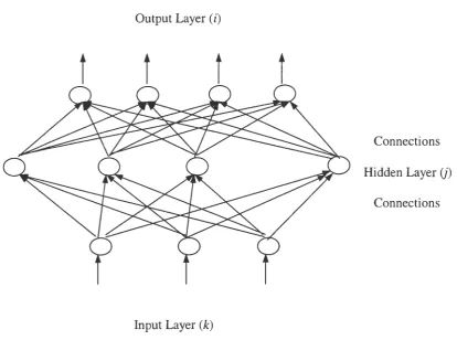
links can form arbitrary topologies. Backpropagation networks is a popular multi-layered,

feed-forward network that consists of input layer, output layer, and at least one hidden layer.

Thus, some units are not directly connected with an outside environment. A typical network

structure for Backpropagation network is illustrated in Figure3, 1.

Backpropagation network is a supervised learning neural network; it receives both the raw

data as input and the desired corresponding output. Typically, it starts out with a random set

of weights and then updates its weights to make it consistent with the examples. This is done

by making small adjustments in the weights to reduce the difference between the observed

and predicted values. In this way, Backpropagation network can minimize prediction and

classification errors incrementally until the network stabilizes. The updating process is

divided into epochs (or cycles). Each epoch involves updating all the weights in the

networks, starting with the output layer and propagating back to the previous layer until the

Output Layer (i)

Connections

Hidden Layer (j)

Connections

Input Layer (k)

Figure 3.1: A Backpropagation network

Backpropagation operates in two phases. Each unit in the neural network has a set of

input links from other units, a set of output links to other units, a current activation level, and

a means of computing the activation level at the next step in time, given its inputs and

weights. In the first operation calledforward-pass, each unit performs a simple computation.

It receives signals from its input links and computes a new activation level that it sends along

each of its output links. The computation of the activation level is based on the values of

each input signal and the weights on each input link. There are two components in the

computation. The first is called input function, in;. that computes the weighted sum of the

in;= I,wj,iaj, j

where W j,i is the weight on link j into node i; a j is the input value of node j.

The second component is called the activation function, g, that transforms the weighted

sum into the final value serving as the unit's activation value, a; :

a . ~ g (in . ).

I I

Usually all nodes in the network apply the same activation function.

In the second operation called backward-pass, differences between the desired and the

actual outputs are propagated back through the network and are used to successively adjust

the layers of the network, beginning with its output layer. If the predicted output for the

single output unit i is O;, and the correct output is T;, then the error is given by Err;= T;

-0; . For Backpropagation networks, there are many weights connecting each input to an

output, and each of these weights contributes to more than one output. Therefore, the trick is

how to divide the error among the contributing weights. The weight update rule for the link

from hidden unit j to output unit i is

Wj,i~ Wj,;+7JX ajxErr;xg' (in;),

where 7] is a constant called the leaning rate, and g' is the derivative of the activation

function. Err; x g · (in;) can be simplified as ~; , which is called the error term of unit i.

The hidden node j is responsible for some fraction of the error ~;; this ~; value is

node, and propagated back to provide the ~ j value for the hidden layer. The propagation

rule for the ~ j value is the following:

Now the weight updated rule for the weights between the inputs and the hidden layer is

almost identical to the update rule for the output layer:

wk

wk

k

where W k,j is the weight of the link between input node k and hidden node j, and I k is the

value of the input node k. Therefore, the algorithm of updating the weights in each epoch

can be summarized as follows:

• Compute the ~ values for the output units using the observed error.

• Start with the output layer and repeat the following for each layer in the network, until

the earliest hidden layer is reached:

1) propagate the ~ values back to the previous layer, and

2) update the weights between the two layers.

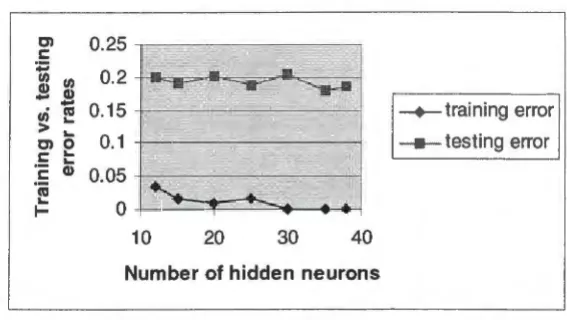
In the real application of Backpropagation networks, through adapting the learning rate 'T/

to the local properties of the error surface, a quick and straightforward convergence of the

gradient descent can be achieved. Oscillations in the proximity of a minimum can be

avoided by introducing a momentum factor a, which accelerates the convergence in wide

plateaus where the gradient is very small. By adjusting other network topology and learning

parameters, such as the number of hidden layers and hidden neurons in each layer, the

3.2 Rule Induction: 1D3 and C4.5

3.2.1 Overview

Inductive learning 1s another popular machine learning technique for classification

domain problems. It is simple, yet powerful, for the problem of classifying a set of variables

into several discrete groups. Unlike neural networks, this method is able to extract a

collection of decision rules from examples expressed on the IF-THEN-ELSE form. These

kinds of rules are more meaningful and accessible to the users. Therefore, it is easier to

maintain and to revise the database. It is also more convenient combine it with human

experts' knowledge.

Iterative Dichotomizer 3 (ID3) algorithm has at its core a procedure based on Hunt's

Concept Learning System (CLS) which, given a set of situations each described in terms of

attributes and a class value, induces a situation classification rule (Quinlan, 1983). Quinlan

adapted an information theory approach in the inductive algorithm where the measure of the

information uncertainty associated with a certain system and the selection of dominant

attributes are perceived as statistical processes. A detailed outline of the ID3 algorithm can

be found in Quinlan (1983).

The ID3 algorithm constructs classification rules in the form of a decision tree

recursively starting at the root. At each node, attribute A is selected to split the training data

into those examples where A = 0 and where A = 1. This algorithm is then invoked

recursively to these two subsets of training data, until all examples in one node belong to the

same class. At this point, a leaf node is created and labeled as the expected value of the

The scheme used in decision tree learning for selecting attributes is designed to minimize

the depth of the final tree. The idea is to pick the attribute that goes as far as possible toward

providing an exact classification of the examples. All we need is a formal measure of "fairly

good" and "really useless." The measure should have its maximum value when the attribute

is perfect and its minimum value when the attribute is of no use at all. One suitable measure

is the expected amount of information provided by the attribute. Information theory is given

as follows: "The information conveyed by a message depends on its probability and can be

measured in bits as minus the logarithm to the base 2 of the probability." Let S be a set of

cases, andfreq(C;,S) stands for the number of cases belonging to class C;. The number of

cases in the set Sis denoted by ISi. If a case is selected at random from a set S of cases and is

announce as belonging to some class C;, this message will have the probability

freq(C;, S)

ISi

and the information it passes on will be

freq(C;, S)

-log ( - - - - ) b i t s .

2 _{IS I}

In general, if we are given a probability distribution S = (p 1 , p 2 , ••• , p" ), where

freq(C;,S)

IS I

then the information conveyed by this distribution, also called the entropy of P, is

k Info (S)

=

-

I

i=I

freq(C;, S)

IS I

freq(C;, S)

* log ( - - - ) bits.

For example, if Sis (0.5, 0.5) then Info (S) is 1, if Sis (0.67, 0.33) then Info (S) is 0.92, if S

is (1, 0) then Info (S) is 0. The higher the entropy of an attribute the more uncertainty there

is with respect to its values.

When this is applied to a set T of training cases, info (T) gives the measure of the average

amount of information needed to identify the class of a case in T. Considering a similar

measurement after T has been partitioned in accordance with n outcomes of a decision test X,

the expected information requirement can be found as the weighted sum over the subsets as

The quantity,

n IT I

info x (T) =

:I-'

-x

gain (X)=info(T) - info x (T),

measures the information gained by partitioning T in accordance with the test X. This

represents the difference between the information needed to identify an element of T and the

information needed to identify an element of T after the value of attribute X has been

obtained, that is, this is the gain in information due to attribute X.

The higher the information gain, the more informative the attribute X. We can use this

notion of gain to rank attributes and to build decision trees where at each node is located the

attribute with the greatest gain among the attributes not yet considered in the path from the

root. Therefore, when a decision tree is being built, the root node of the tree would

correspond to the attribute with the lowest entropy value and the highest gain value.

The intent of this ordering is two-fold:

1) To create small decision trees so that records can be identified after only a few questions.

Although the gain criterion gives good results, it has a serious problem: there is a strong

bias in favor of decision tests with a greater number of outcomes. This bias inherent in the

gain criterion is rectified by a kind of normalization in which the apparent gain attributable to

tests with a greater number of outcomes is adjusted. Consider the information content of a

message with regard to a case that gives the outcome of the test rather than the class to which

the case belongs. Analogous to the definition of info (S), it can be defined as

~IT.I IT.I

Split info (X) = L i - ' xlog2 ( - ' ),

i=I ITI ITI

where split info (X) represents the potential information generated by dividing T into n

subsets, whereas the information gain measures the information relevant to the classification

that arises from the same division. Then

gain(X)

gain ration (X) =

-split inf o(X)

expresses the proportion of information generated by the split that is useful, i.e., that appears

helpful for classification.

3.2.2 C4.5

C4.5 is the direct descendent of ID3 and was developed by Quinlan as well. It accounts

for unavailable values, continuous attribute value ranges, pruning of decision trees, rule

derivation, and so on. Similar to ID3, C4.5 is able to create a classifier in the form of a

decision tree consisting of leaves and decision nodes. The leaf indicates a class and the

decision node contains some test to be carried out on a single attribute value. This will result

contains heuristic methods for simplifying (pruning) decision trees, with the aim of

producing more comprehensible structures without compromising accuracy on unseen cases.

In building a decision tree, C4.5 can deal with training sets that have records with

unknown attribute values by evaluating the gain ratio for an attribute by considering only the

records where that attribute is defined. In using a decision tree, C4.5 can classify records that

have unknown attribute values by estimating the probability of the various possible results.

C4.5 can deal with the case of attributes with continuous ranges as follows. Say that

attribute C; has a continuous range. The training cases T are first sorted on the values of the

attribute C;. There are only a finite number of these values denoted in increasing order, A 1 ,

A 2 , ••. , Am . Then for each value A j , j= 1, 2, ... , m, we partition the records into those that C;

have values up to and including A j (e.g., A 1 to A j ) and those that have values greater than

A j ( e.g., A j+I to Am). For each of these partitions we compute the gain ratio and choose the

partition that maximizes the gain.

There is a very general phenomenon called overfitting for the decision tree learning

algorithm. It happens when the algorithm uses the irrelevant attributes to make spurious

distinctions among the examples, while the vital information is missing. Pruning of the

decision tree is a way to treat the overfitting done by replacing a whole subtree by a leaf

node. The replacement takes place if a decision rule establishes that the expected error rate

in the subtree is greater than in the single leaf. Start from the bottom of the tree and examine

each nonleaf subtree. If the replacement of this subtree with a leaf, or with its most

frequently used branch, were to lead to a lower predicted error rate, then the tree would be

Since the error rate for the whole tree decreases as the error rate of any of its subtree is

reduced, this process will lead to a tree whose predicted error rate is minimal with respect to

the allowable forms of pruning. The additional computation invested in building parts of the

tree that are subsequently discarded can be substantial, but this cost is offset against benefits

due to a more thorough exploration of possible partitions. Growing and pruning trees is

slower, but more reliable.

3.3 Rough Sets

3.3.1 Overview

Rough set, proposed by Pawlak in the early 1980s (Pawlak, 1982, Pawlak, 1991), is a

mathematical approach used to deal with data analysis and knowledge discovery from

imprecise and uncertain data. The starting point of this theory is that objects may be

indiscernible in terms of the value of attributes. A rough set is a set of objects which cannot

be precisely characterized based on the set of available attributes. In this case, any vague

concept in the rough set is replaced by a pair of lower and upper approximations. These two

approximations are two basic operations in the rough set theory.

3.3.2 Basic Concepts

3.3.2.1 Knowledge Representation System (KRS)

As data representation framework employed in the rough set theory, knowledge

representation system is a finite table, with rows labeled as objects, columns labeled as

attributes, and entries of the table called attribute values. It is also known as information

system. A formal definition of KRS is given below.

Let S = < U, Q, V, f > be a KRS, where U is a non-empty, finite set of objects, the

set of condition attributes C and a non-empty set of decision attributes D. We have Q = C

u

D and C n D = <I>. V =

U

and the elements of V q are called values of the attribute of q. f is the information function

that assigns a unique value of the attribute q to each object u; EU.

3.3.2.2 Indiscernible Relation

Suppose Pis a non-empty subset of Q, u; and u j are members of U. We can associate an

approximation space in S by defining a binary indiscernible relation as follows:

IND (P) = { (u;,

u)

We say that u; and u j are indiscernible or equivalent by a set of condition attributes P in S

IFF V qE P, f (u;, q) = f (u j , q). This indiscernible relation partitions U into several

elementary sets. Each elementary set in IND (P) consists of a group of objects which has the

same value of attributes; thus u; and u j are in one elementary set in terms of the attribute

subset P.

3.3.2.3 Approximation of Set

Based on the concept of indiscernible relation, a universe U can be divided into several

elementary sets by any subset of the attribute Q.

Suppose Xis a non-empty subset of C. U is divided into A= {A1 , A2 , ••• ,A;} in terms

of X and divided into D = { Di, D2 , ••• ,D j} in terms of D. For each class D n (n=l, 2, . .. ,j)

in D:

• If all objects in Am (m=l, 2, ... , i) are contained within D n , we say Am is in the

• If no object in Am (m= 1, 2, ... , i) is contained within D n , we say Am is in the negative

region of D n , that is NEG (D n ).

• If some objects in Am (m= 1, 2, ... , i) are contained within D n , we say Am is in the boundary region of D n , that is BND (D n ).

The lower approximation of set D n , denoted by X D n , is the union of all Am in the

positive regions. The upper approximation of set D n , denoted by X D ,,_, is the union of all

Am in the positive regions and boundary regions.

We say that the lower approximation consists of all objects belonging to the concept D n and the upper approximation consists all objects which possibly belong to the concept. Any set D n (n=l, 2, ... , j) that has a non-empty boundary region is called rough, since it can be

characterized only approximately. 3.3.2.4 Dependency of Attributes

The dependency of attributes is the relationship between condition attributes C and decision attributes D. Analysis of dependency is used to determine whether D can be characterized by the value of C. It is of primary importance in the rough set approach to discover data regularities for deriving rules.

The dependency of the decision attribute (D) on the condition attributes (C) equals the ratio of the number of objects in the positive regions to the number of objects in the universe U. It can range from O to 1 :

• It is between O and 1 when there is a partial dependency between C and D, i.e., only

some objects can be classified into some categories of D based on the attributes in C.

3.3.2.5 Reduction of Attributes

Another important issue is the identification and elimination of redundant conditions.

The objective is to find a subset of attributes that have the same discriminating power as the

set of original attributes without losing any essential information. After all redundant

attributes have been eliminated, the remaining subset of attributes is called a minimal subset

or reduct.

Reduct R is defined as a minimal subset of attributes remaining the same degree of

dependency between C and D, and none of the attributes in R can be further removed without

affecting the degree of discerning power. For each reduct, we can derive a reduct table from

the original knowledge representation system by removing those redundant attributes.

3.3.2.6 Decision Rule

3.3.2.6.1 Decision Rule Generation

Decision rules are generalized based on the non-redundant attributes contained in the

chosen reduct. Values for these attributes are then analyzed to identify patterns in the data.

The patterns are then expressed as logical statements which link the value of specific

conditions with an outcome. A typical rule is:

If conjunction of elementary conditions ( Cond_C),

The elementary condition formulae over subset X ~ C and domain V xi of attribute

xi E X are defined as: xi= vi, where vi E V xi. By Cond_C we denote a conjunction of

elementary condition formulae, i.e. (x 1 = v 1 ) /\ (x 2 = v 2 ) /\ ••• /\ (x, = v,) for all xi E X.

Similarly, we define elementary decision formulae d = v j , where v j EV D by Dec_D.

We denote a disjunction of elementary decision formulae, i.e., (d = v 1 ) /\ (d = v 2) /\ •.• /\ (d

= vs). If s equals 1, there is only one elementary decision in Dec_D and the rule is certain

rule. Otherwise, there are several elementary decisions in Dec_D, and the rule is a possible

rule. This means available conditions Cond_ C cannot exactly discriminate between

elementary decisions.

The strength of decision rule is the number of objects satisfying Cond_ C and belonging

to one of the decisions in Dec_D. In possible rules, strength is calculated for each decision

elementary separately.

The decision rules can be employed to analyzed new objects and partition them into

different classes. If new object matches one possible rule, strength for all suggested decision

classes in Dec_D in this rule will be assessed and the new object will be included into the

class with the most strength.

3.3.2.6.2 Evaluation of Decision Rules

There are several measures used to evaluate the performance of decision rules.

1) Accuracy of decision rule

The accuracy of a rule with respect to a specific decision value can be defined as the ratio

matching rule conditions. Rules with high accuracy are usually desirable because the probability of an error is smaller.

2) Decision coverage

The decision coverage for a certain class equals the percentage of all cases with a matching rule decision and covered by rules for this decision to the number of cases with the decision value. An optimal set of rules is one which has acceptable values of rule strength, rule accuracy and decision coverage. However, the process of optimization may involve some trade off. To increase rule strength or decision coverage, one may have to decrease the accuracy of rules.

3.3.3 Advantages of Rough Set

The advantages and potential applications of the Rough Sets theory have been presented by Dimitras et al. (1999), Hashemi et al. (1998), Nagaraja (1997), Pawlak (1997), Pawlak et al. (1995), Slowinski et al. (1997), and Szladow and Ziarko (1993). It has been successfully applied for knowledge acquisition, forecasting and predictive modeling, decision support, etc.

• The main advantage is that it does not require any preliminary or additional information about the data.

• The method allows work with incomplete data without replacing missing values, to switch between different reducts, to use less expensive or alternative sets of measurements.

• It offers the ability to handle large amounts and various types of data.

• Since the rules generated and attributes used are non-redundant, the patterns are very

compact, strong, and robust.

• The ability to model highly non-linear or discontinuous functional relationships provides

a powerful method for characterizing complex, multidimensional patterns.

• Rough sets can identify and characterize non-deterministic systems and incorporate

probabilistic information and decision--making.

3.4 Summary

In this chapter, we reviewed three artificial intelligence techniques we would use in the

experiment. In the past several years, there have been several studies, which compared the

performances of either two of these three technologies or combined them as a hybrid system.

Mooney et al. (1989) found that ID3 was faster than a Backpropagation net, but the

Backpropagation net has stronger power to noisy data. Because of the rules created in the

forms of decision trees, it is easier to explain the output values created by using rule

induction methods. While to the Backpropagation net, it is relatively difficult to explain the

output based on those weights between neurons. Dietterich et al. (1995) stated that the

performance of these two techniques depends on the decoding method employed to the

CHAPTER4

COMPARISON OF PERFORMANCES OF THREE METHODS

4.1 Preparation and Experiment

4.1.1 Data Description

The system call data set used in this experiment was from the immune system web site.

It is for one privileged program - sendmail. The details of generating the sendmail traces

used in this experiment were given in (Hofmeyr 1998) and on the immune system web site.

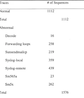
The data includes several traces:

• Normal traces: a trace of the sendmail daemon and several invocations of the sendmail

programs. During the period of collecting these traces, there were no intrusions or any

suspicious activities happening.

• Abnormal traces: several traces either including intrusions or dangerous attempts. There

are five error conditions of forwarding loops, three sunsendmailcp attacks, two traces of

the syslog-remote attacks, two traces of the syslog-local attacks, two traces of the decode

attacks, 1 trace of the sm5x attack attempt and one trace of the sm565a attack attempt.

The descriptions of these intrusions can be found on the web site.

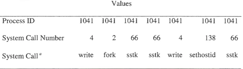
Each trace has one or more processes of sendmail programs, so each trace has two

columns of data, the first one is the process ID indicating which process the system call

belongs to and the second one is the system call value. In previous research, system calls

were converted from string to integer values for ease of computing. Because there are totally

182 kinds of system calls considered, the values of system calls ranged from O to 181. The

index about the numeric values and their related system call names can be also found on the

Table 4.1: An example of the Sendmail Trace.

Process ID

System Call Number

System Call a

Values

1041 1041 1041 1041 1041 1041 1041

4

2

66

66

4

66

write fork sstk sstk write sethostid sstk

a The system calls in last row will not appear in the data set.

to one process. In this sequence, "write" is the first system call, and "sstk" is the last one.

4.1.2 Data Preparation

Based on previous research, short sequences of system calls made by a program during

its normal executions are very consistent and can be used for anomaly detection. Our

purpose is to recognize the different patterns of normal and abnormal behaviors by using

various learning algorithms. First, we need to set up these sequences from the original data

sets. We have one system call and N-1 subsequent system calls in the same process compose

one sequence of length N.

We suppose that all sequences of system calls from normal traces should be normal

sequences, while those from suspicious traces which cannot be found in the normal traces are

abnormal sequences. Using a sliding window of length N, we can search through all the

traces and set up two data sets, one consists of normal sequences and another consists of

abnormal ones. In previous research (Hofmeyr et al., 1998), the proper length of sequence

tested varied from 2 to 30. The conclusion of the research was that the length of the