Intelligent Load Management Scheme for a Residential
Community in Smart Grids Network Using Fair
Emergency Demand Response Programs
Muhammad Ali1, Zulfiqar Ali Zaidi2, Qamar Zia3, Kamal Haider4, Amjad Ullah3, Muhammad Asif5 1Electrical Engineering Department, COMSATS Institute of IT, Abbottabad, Pakistan
2Department of Mathematics, COMSATS Institute of IT, Abbottabad, Pakistan
3Electrical Engineering Department, NWFP University of Engineering & Technology, Peshawar, Pakistan 4Electrical Engineering Department, Gandhara University, Peshawar, Pakistan
5Electrical Engineering Department, CECOS University of IT, Peshawar, Pakistan Email: [email protected]
Received May 25,2012; revised June 27, 2012; accepted July 10, 2012
ABSTRACT
In the framework of liberalized deregulated electricity market, dynamic competitive environment exists between wholesale and retail dealers for energy supplying and management. Smart Grids topology in form of energy management has forced power supplying agencies to become globally competitive. Demand Response (DR) Programs in context with smart energy network have influenced prosumers and consumers towards it. In this paper Fair Emergency Demand Response Program (FEDRP) is integrated for managing the loads intelligently by using the platform of Smart Grids for Residential Setup. The paper also provides detailed modelling and analysis of respective demands of residential con-sumers in relation with economic load model for FEDRP. Due to increased customer’s partaking in this program the load on the utility is reduced and managed intelligently during emergency hours by providing fair and attractive incen-tives to residential clients, thus shifting peak load to off peak hours. The numerical and graphical results are matched for intelligent load management scenario.
Keywords: Demand Response (DR); Fair Emergency Demand Response Program (FEDRP); Intelligent Load
Management (ILM); Residential Area Networks (RAN); Smart Grids
1. Introduction
The electric industry is poised to make the renovation from a centralized, producer controlled net-work to one that is less centralized and more consumers interactive. The advancement to smarter grid promises to change the industry’s intact business model and it will be beneficent to all i.e. utilities, energy service providers, technology automation vendors and all consumers of electric power.
SG brings improvement in the existing electric grid by incorporating intelligence to each single grid component and the grid architecture. In Residential Area Network (RAN), there is energy manager called REM communi-cates with Home Energy Manager (HEM) through wire-less technology IEEE 802.16. The REM updates the cus-tomers about demand response programs, the peak hours, off peak hours etc. through Smart Meters (SM). In [1], author mentioned that in Home Area Network (HAN), home appliance including electric vehicle chargers, secu-rity products, refrigerators, microwave, and air condition-ers etc. communicates with each other and HEM using
Zigbee technology. In [2], authors suggested Zigbee for home automation due to its low power consumption, low cost, a lot of network nodes and reliability.
Time Pricing. In market based programs, participation in the programs are given cash for the load reduction during critical hours.
The paper is divided into six broad sections in which second section highlights related work and third section focuses on problem formulation. Fourth section shows detailed model and analysis of FEDRP under the concept of residential area networks and is subdivided into five sub sections. Fifth section shows all numerical and graphi-cal analysis in detail and last section shows conclusion of the work.
2. Related Work
Recently energy management is an active topic due to continuous rise in global energy consumption continuously [5]. As a result, the existing electricity grid is expected to experience difficulties in generating the necessary power for large amounts of increasing load, distributing the re-quired power and keeping the generated power and the load balanced. As in [6], the participation in DR programs is helpful in customer bill reduction as they reduce load during peak hours as their normal consumption is less than their class average.
During the peak hours, the load on the grid increases than the base load. As mentioned in [7], it is not possible for a power plant to generate adequate power at peak load level and store it when the load is lower, backup plants are used to accommodate the peak loads. Thus these plants incur extra cost for the utility due to extra generation to convene load demands. To compensate the cost, the pro-sumer has to increase the cost of unit which reduces cus-tomer participation during peak hours. The load manage-ment techniques are used to reduced peak demands in order to reduce the burden from the grid [8].
For REM different appliances scheduling schemes have also been proposed to reduce the load in SG. In [9], the authors use the particle optimization technique to sched-ule demands in an automated way. In [10], authors re-duce the peak to average electricity usage ratio by Opti-mal Consumption Schedule (OCS) for the customers in a neighbourhood. The authors in [11], an optimized REM algorithm is proposed that is helpful in reducing the peak load in which appliance start period is scheduled. In [12], an automatic controller design is suggested that schedule appliances to provide an optimal cost. A neural network base prediction approach has been proposed in [13], to optimize the schedule of micro CHP devices. In [14], an energy management protocol is proposed in which con-sumer sets maximum consumption value and the residen-tial gateway can turn off the device in standby mode.
In [15], Emergency Demand Response Program, is used as a method for Available Transfer Capability enhance-ment, and this implementation is evaluated from both eco-nomical and reliability view points. For this aim, the Emer-
gency Demand Response Program is implemented for specific loads which are chosen according to a sensitivity analysis.
3. Problem Formulation
Smart grid advent brings challenges with opportunities for the end-users and utility. EDRP is one of incentive based program which is offered to consumer to reduce their loads during peak hours [16-18] by giving them incentive payments. In residential area networks (RAN) customer response is totally dependent upon program associated cost; if price is high it must effect customer participation in certain program. In EDRP end user are charged at high prices during peak hours than off-peak hours for any load either “must run” load or “optional” loads, it results in less consumer participation which ultimately cause less revenue generation for utility. Although incentives attract users to cut down their demand during peak hours, but in any case user has to pay high price for must run and vari-able loads during peak hours.
The scope of this paper is to incorporate fairness in existing EDRP to sustain stability between utility and end- user. Fairness means to make DR programs more reliable and viable, the author in [19] gives idea about clustering based on different categories and shows how customer’s participation can be enhance in DR programs, also differ-ent schemes are described in [20] for load managemdiffer-ent This article mainly focuses on how fairness can be amal-gamate in RAN for this article suggests the concept of Fair emergency demand response program (FEDRP). In residential setup load can be categorized by author in as fixed or “must run” load and variable or “optional” load. In existing EDRP fixed and variable loads are charged at same price during peak and off peak hours which cause less consumers participation and satisfaction. In proposed FEDRP customer must be provided same prices in peak and off peak hours for fixed or “must run” loads and only variable or optional loads prices are time variant from peak to off-peak; and also incentive will be offered end users for cutting down their loads during peak hours. This article provides best possible solution for achieving maximum end user participation and to reduce the loads during peak hours.
4. Modeling and Analysis of FEDRP
4.1 Fixed and Variable Load Economic Model for RAN
cus-
tomer involvement, demand of customer is to be analyze against change in prices for must run and optional loads. The price elasticity of demand is defined as the proportion of change in demand to the change in price.
a a
d p
p d
e d p (1)
t t
p p
y x
d i d i
tt
e (2)
t t
p p
y x
d i d i
tt
e (3) Logarithmic modeling of elastic load:
If customer demand changes based on incentive offered by utility so;
d iy
d ix
d ix d iy
d i
(4) The prize incentive attracts the consumer so total in-centive INC (Δdt) function is given as;
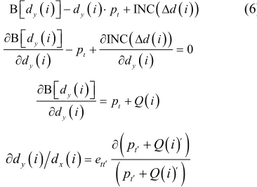
INC d i Q i (5) Customer benefit for participating in DR program will be;
tINC
d i
Bd iy d iy p
(6)
B y IN
t d i p d i
C
0 y y d i d i
B t d ip Q i
y
y
d i
t
tt t
p Q i
p Q i
e t
y x e
d i d i
By assuming constant elasticity for NT hours period, tt is equal to constant for and NT
t integration of each term we obtain following relation.
0 d NT 1 0 d d ( ) t t y x i x Q i p t tt t p e i i pp Q i
dyi
t t
Q i
p Q i
(7)Combining the optimum customer behavior that leads to
NT
2
1Ln
x x t
t
d i d i p Q i p 0
tt
y
e t t
d i
p Q i
(8)Parameter η is DR potential which can be entered to model as follows:
2 NT 0 1 Ln y e
x x t t t
t
d i
d i d i p Q i p p Q i
tt
(9)Larger the value of η means the more customer tendency to reduce or shift consumption from one hour to the other. 4.2. For Fixed Loads
For non shift able or must run loads we have elasticity known as “self elasticity” as [10] describes it.
0 s s s d e p (10)
As in our FEDRP must run loads price remain fixed and invariant of peak and off-peak hours so demand at any time for must run (base) loads will be given as
y x
d i d i (11) So, demand for base loads will remain same through peak and off-peak hours and eventually customer’s par-ticipation increases in FEDRP.
4.3. Cost of Customer Participation
FEDRPC d ix d iy Q i
(12) 2 1 FEDRP , C T tQ i e t t
p t
h f v
D d d
4.4. Demand Modeling of RAN
In a residential setup demand of electricity vary with con-sumer level, for a same price at some definite interval demand of a home may be different from other home. In our proposed FEDRP demand (Dh) of consumer is
alien-ated into two portions, must run loads demand (df) and
optional load demand (dv);
p p p p
hd hc hb ha
D D D D
1a 2a 3a 4a
ha
D d d d d
(13) In Figure 1(a) price of electricity is changing with the
demand for variable loads with change in price in such a way that 1 2 3 4. d1 is demand of customer during peak hours where price increases which ultimately result in less customer’s demand and for d2, d3 and d 4 end user’s demand is increased due to decreased prices, and for fixed loads as described in Figure 1(b) price remain
same during peak and off peak hours.
In Figure 2 residential area setup is modeled such that
demand of consumers is varying such that:
[image:3.595.102.285.379.512.2](a)
(b)
Figure 1. (a) Demand and price curve for optional (variable) loads; (b) Demand and price curve for fixed (must run) loads.
6 14
1 2
1 7
a a hb
i i
D d d
20 3 24 415 21
a a i i
d d
20 24
3 4
15 21
b b i i
d d
(16) where “i” determine the period of time that customer demand during interval d1, d 2, d 3, and d 4.
Now for second home demand considering both optional and must run load will be:
6 14
1 2
1 7
b b hb
i i
D d d
[image:4.595.60.280.71.559.2]
(17) Similarly demands of home three and four are given as:Figure 2. Demand and price curve for variable loads four homes in RAN.
6 14 20 24
1 2 3 4
1 7 15 21
c c c c hb
i i i i
D d d d d
6 14 20 24
1 2 3 4
1 7 15 21
d d d d
hb
i i i i
D d d d d
(18)
6
1 1 1 1
1 14
2 2 2 2
7 20
3 3 3 3
15 24
4 4 4 4
21
a b c d
f f f f
i
a b c d
f f f f
i f
a b c d
f f f f
a b c d
f f f f
d
d d d d
d d d d
d d d d
d d d
d
(19) So the total fixed demand and variable demand for RAN during 24 hours is given as;
14
7 20
15 24
21 6
1 1 1 1
1
2 2 2 2
3 3 3 3
4 4 4 4 i
v
a b c d
v v v v
i
a b c d
v v v v
a b c d
v v v v
a b c d
v v v v
d
d d d d
d d d d
d d d d
d d d d
(20)
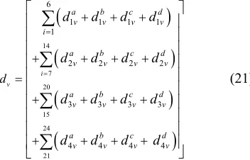
Above equation describes the fixed demand in RAN during 24 hours similarly variable demand during a day is expressed as;
(21)
[image:4.595.360.536.592.705.2]hb hc hd
D D D
h f v
D d d
1 1 2 2 3 3 3 3 4 4 c c f v b b f v a a f v d d f v c c f v d d d d d d d d d d able or “optional” loads. This means that revenue and bene-fit of utility will be given as:
t ha
D D (22)
As total demand is equal to total fixed and total vari-able demand
61 1 1 1
1
14
1 1 7 2 2
20
2 2 2 2 15
3 3 3 3
24
4 4 4 4
21
4 4
a a b b
f v f v
i
d d a a
f v i f v
c c d d
f v f v
t b b c c
f v f v
a a b b
f v f v
d d
f v
d d d d
d d d d
d d d d
D
d d d d
d d d d
d d
(23)By simplifying above equation, so total demand of these homes in residential setup from (16), (17), (18), and (19) will be:
t ha
D D DhbDhcDhd
4
2 2 2
7
4 4
a b c d
a b c d
d d
d d d
1 1 2 2 3 3 4 d m d m d m m d d d d d d d ( , )R f p d
In proposed model company revenue is of two types, first that utility obtain from fixed or “must run” loads and other revenue from variable or “optional” loads. This means that revenue will be given as:
6 1
1 1 1 1 2
1
20 24
3 3 3 3 4 4
15 21
t
a b c d
i i
a b c d
D
d d d d d d
d d d d d
(24)Considering total demand for residential setup of “m” homes with different demands during “4” intervals in 24 hours is described as
6
1 1 1
1 14
2 2 2
7 20
3 3 3
15 24
4 4 4
21
a b c
t i
a b c
i
a b c
a b c
D d d d
d d d
d d d
d d d
(25)Equation (22) shows the total demand of “m” homes during 24 hours at four different intervals.
4.5. Utility Revenue
Scope of this article is to increase utility revenue along with the maximum customer satisfaction. In FEDRP util-ity revenue is of two types, first that utilutil-ity obtain from fixed or “must run” loads and other revenue from vari-
f v
R R R
1 1 1 1
3
0 0 0 0 0
d d d d
a b c d
i i i i
d d d d
f i
R p D D D D
(26) Taking into consideration the demands of four homes and their respective revenues at four intervals is calculated as:
Revenue from fixed (must run) loads will be:
1 1 1 1
3 1
0 0 0 0 0
d d d d
a b c d
i i i i
d d d d
v i
i
R p D D D D
(27)
Revenue from variable (optional) loads will be:
1 1 1 13
1
0 0 0
0 0
d d d d
a b c d
i i i i
d d i
i
d d
R
p p D D D D
(28)
Using Rf, Rv in (23):
1 u k k (29)For “m” homes revenue to utility at four intervals is described as (see Equation (30), below)
Benefit function for utility is given as: Profit = Revenue – Total operating cost
y R G C
1 1 1 13
1
0 0 0 0
0
1
d d d d
a b c d
i i i i
i d i u d d k k d
y p p D D D D
G C (31)
(35. Numerical Results and Simulation
has been
1 1 1 1 13
1
0 0
0 0 0 0
d d d d d
a b c d m
i i i i i
d d d
i i
d d
R p p D D D D D
2)
In this section numerical and graphically study
evaluated considering FEDRP. For this purpose daily load curve of Pakistani local grid has been taken for this simula-tion studies. The curve is divided into three secsimula-tions as low load, off load and peak load periods as shown in Table 1
and energy prices are taken in rupees in different periods.
[image:5.595.315.539.250.430.2]The selected values of self and cross elasticity’s have been shown in Table 2.
Fairness index has been calculated for fair emergency demand response program as follows;
Fairness index (FI) in [4] is described as ratio of cus-tomers whose demand is satisfied to total number of
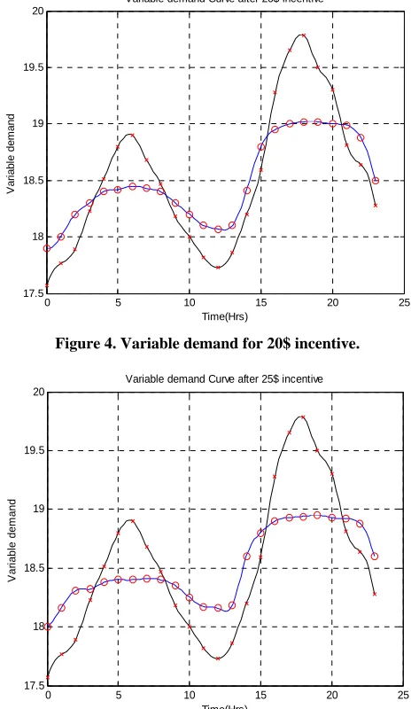
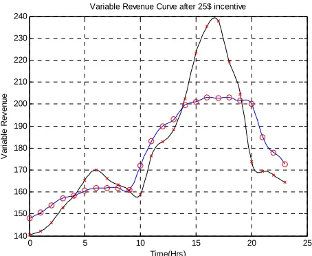
has been analyzed in these figures that energy of daily load during peak hours has been sufficiently reduced and is shifted to off peak periods. Giving more incentives has permitted consumers to shift th
period. Similarly, Figures 6-8
erated for utility company offering the program under
dif-ferent cases le revenues
generated to ation using
their variable loa n ca umeri and analyzed graphically emonstrated in Figure . In
all the analysis cases ncentives a ompare
wit centive cases which e the w ce- nario
customers. Utility should effectively manage the cus-tomers demand weather for must run or optional loads. Fairness index given as:
1 f 1 v
i i
FI
a a
d d
ad demand of 40 customers are satisfied and optional needs for 30 customers satis-fied, and also priority of fixed load is twic
load [6], then FI = 0.91. The client contentment for no
(33)
where β, γ are the priority of different loads and α is number of total customers. Considering the case for ex-ample in peak hours fixed lo
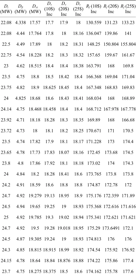
e of optional mandatory load depends on price variation for this load during peak and off-peak hours. Higher the prices less will be the demand of customer, for satisfying its optional load. Total numerical analysis of daily load curve has been evaluated in Table3 which shows utility fixed and
vari-able revenues (Rf and Rv) under different cases of
incen-tives given to clients for program participation. Initial fixed and variable demands (Dfi and Dvi) for the utility is shown
with zero dollar incentives but the important thing is that as giving 25 dollar incentive for peak reduction to clients, Dv shifts tremendously as compared to 10 and 20 dollar
incentives.
Totalenergy and peak reductions have been calculated in Table 4.
Figures 3-5 show the total variable demand analysis
[image:6.595.309.539.268.735.2]when different cases of consumer participation have been taken under different scenarios of incentives given by the utility company to those customers who sign up the contract for FEDRP. Incentives in the form of 10, 20 and 25 dollars are given to the participants to reduce their variable load during emergency or peak hour. It
Table 1. Energy prices of daily load curve.
Low-Load Off-Period Peak
Period (HRS) 00:00 am to 9:00 am 09:00 am to 5:00 pm 5:00 pm to 00:00 am
Energy Prices
[image:6.595.55.288.588.740.2](per KWH) 6 Rps 8 Rps 10 Rps
Table 2. Self and cross elasticity’s.
Low Load Off-Peak Peak
Low Load –0.1 0.01 0.012
Off-Peak 0.0
eir load to off peak show fixed revenues of incentives. The cases of variab
utility from customer’s particip d has bee lculated n cally
as d s 9-11
of i re c prov
d clearly hole s h non in
.
Table 3. Total numerical analysis of load curve. Di
(MW) (MW)Dfi (MW)Dvi Dv
(10$) Inc
Dv
(20$) Inc
Dv
(25$) Inc
Rf(10$)
Inc Rf(20$) Inc Rf (25$)Inc
22.08 4.338 17.57 17.7 17.9 18 130.559 131.23 133.23
22.08 4.44 17.764 17.8 18 18.16 136.047 139.86 141
22.5 4.49 17.89 18 18.2 18.31 148.25 150.804 155.804
22.75 4.54 18.228 18.2 18.3 18.32 157.65 159.67 161.67
23 4.62 18.515 18.4 18.4 18.38 163.791 168 169.8
23.5 4.75 18.8 18.5 18.42 18.4 166.368 169.04 171.04
23.75 69.83
4 1
24.14 4.75 18.468 1 8 168.712 167.978 167.778
23.92 4.71 18.18 18.28 18.3 18.35 169.89 168 166.68
23.72 4.73 18 18.1 18.2 18.25 170.671 171 170.5
23.5 4.74 17.82 17.9 18.1 18.17 171.228 173 174.4
23.65 4.78 17.73 17.83 18.07 18.16 172.45 173.68 174.5
23.8 4.8 17.86 17.92 18.1 18.18 173.02 174 174.3
24 4.84 18.2 18.28 18.41 18.6 173.765 173.8 173.8
24.2 4.91 18.59 18.6 18.8 18.8 174.87 172.78 172
24.7 4.92 19.279 19.13 18.95 18.9 175.176 172.359 171.89
24.5 4.94 19.65 19.25 19 18.93 175.368 172.616 171.616
25 4.92 19.785 19.3 19.02 18.94 175.341 172.621 171.621
24.7 4.92 19.5 19.28 19.018 18.95 175.29 173.6491 172.1
24.5 4.87 19.305 19.24 19 18.93 174.813 176 176
24.3 4.85 18.815 18.915 18.99 18.92 174.54 175.92 176.92
24.15 4.78 18.64 18.84 18.876 18.88 174.22 175.86 177.4
23.7 4.75 18.275 18.375 18.5 18.6 174.162 175.78 177.6 4.82 18.9 18.625 18.45 18.4 167.348 168.83 1
1
Peak 0.012 0.016 –0.1 –0.1 0.016
24 .825 8.68 18.6
8.45
18.43
18.4 18.41
18.4
[image:6.595.55.290.590.647.2]C
Rv (10$) Inc R (20$) Inc R (25$) Inc ontinued
v v
143 147
20
148
144.612
147.48 153 154
2
159.8 160 160.5
1
161. 2 12 161.
183 183
215. 205.
204. 200.
168. 5 170. 5 172. 5
148.612 150.612
154.2 156. 157.2
156.4 158.3 158.3
162.2 16 161.7
162.12 162.52 161.92
21 160
161.82
161
8212 161
161 168 172
180 184.76 189.32
188.76 190 193 193
208.4 200.4
206.
199.4
214.08 08 201.08
216.9 207 203
217.8 207.6
5 203.
202.6
065 06 065
210.5 5 201.5
180.745 0012 200.0012
174 180 185
170 175 178
57 57 57
[image:7.595.305.538.86.276.2]redu
Table 4. Ene gy and peak tions in % w ifferent scenar
Differen Cas
otal Energy
MWhr Reduction
Peak (MW)
eak ction
)
r ios.
c ith d
t Inc T es
Energy
(%)
P Redu
(%
(0$) Inc 580 0 24.7 0
(10$) I 575 0. 24.5 9717
(20$) 568 24.09 636
(25$) I 566.89 2. 23.9 8866
nc 862069 0.80
Inc 2.068966 2.469
nc 260345 3.23
0 5 10 15 20 25
17.5 18 18.5 19 19.5 20
Variable dem ter 10$ incentiv
Time(Hrs)
V
a
ri
ab
l
[image:7.595.306.538.89.489.2]m
Figure 3. Variable demand for 10$ incentive. and Curve af e
e
de
and
0 5 10 15 20
19.5
19
18.5
18
17.5
Variable demand Curve after 20$ incentive
Time(Hrs)
V
ar
iabl
e d
em
a
nd
25
Figure 4. Variable demand for 20$ incentive.
20
5 10 15 20
19.5
19
18.5
18
17.5
0 25
Variable demand Curve after 25$ incentive
V
a
ri
ab
le de
m
an
[image:7.595.57.283.99.406.2]d
Figure 5. Variable demand for 25$ incentive. Time(Hrs)
180
5 10 15 20
175
170
165
160
155
150
145
140
135
130
0 25
Fixed Revenue Curve after 10$ incentive
F
ixe
d
R
e
ve
n
u
[image:7.595.55.288.442.717.2]e
[image:7.595.311.537.517.716.2]0 5 10 15 20 25 130
135 140 145 150 155 160 165 170 175 180
Fixed Revenue Curve after 20$ incentive
Time(Hrs)
F
ix
ed R
ev
e
nue
240
230
220
210
200
190
180
170
160
150
140
0 5 10 15 20 25
Variable Revenue Curve after 20$ incentive
Time(Hrs)
V
ar
iabl
e R
ev
[image:8.595.310.538.84.275.2]enue
[image:8.595.61.289.86.277.2]Figure 10. Variable revenue for 20$ incentive. Figure 7. Fixed revenue for 20$ incentive.
0 5 10 15 20 25
130 135 140 145 150 155 160 165 170 175 180
Fixed Revenue Curve after 25$ incentive
Time(Hrs)
F
ix
ed R
ev
enu
[image:8.595.61.288.302.495.2] [image:8.595.310.537.303.489.2]e
Figure 8. Fixed revenue for 25$ incentive.
0 5 10 15 20 25
140 150 160 170 180 190 200 210 220 230 240
Variable Revenue Curve after 10$ incenti
Time(Hrs)
V
ar
iabl
e R
ev
enue
ve
Figure 9. Variable revenue for 10$ incentive.
V 240
230
220
210
200
190
180
170
160
150
140
0 5 10 15 20 25
ariable Revenue Curve after 25$ incentive
Time(Hrs)
V
a
ri
ab
le
R
e
v
e
nu
e
6. Conclusion
In this paper utility revenue and profit is modeled con-sidering RAN for different user levels consumption, also demand of consumer is modeled mathematically and gra- phically. As consumer participation and satisfaction in DR program is basic tool to measure competitiveness for any DR program in market, so in this article end user par-ticipation is represented graphically with the comparison of initial demand before FEDRP. For customer content-ment fairness index of the FEDRP is also calculated. De-mand curve of FEDRP is plotted and also modeled nu-merically and compared with the existing EDRP.
7. Acknowledgements
The special thank goes to Dr. Imdad and Mr.
Waheed-ur-Reham
prepa-ration ful to
Figure 11. Variable revenue for 25$ incentive.
[image:8.595.61.288.523.715.2]Mr. Abdul Rehman as they have
of Markets,” Electric Pow
, 2008, pp. 1989-1996.
19-21 January 2010, pp. 1-6.
[11] M. Erol-Kantarci, “Wireless Sensor Networks for Cost- Efficient Residential Energy Management in the Smart Grid,” IEEE Transactions on Smart Grid, Vol. 2, No. 2, 2011, pp. 314-325.
Mr. Istiaq Khan and made
a great contribution throughout our work especially in editing the text and paper formatting.
REFERENCES
[1] J. Pelletier, “ZigBee Powered Smart Grids Coming to a Home near You?” 2009.
[2] Z. Md. Fadlullah, M. M. Fouda, N. Kato, A. Takeuchi, N. Iwasaki and Y. Nozaki, “Toward Intelligent Machine- to-Machine Communications in Smart Grid,” IEEE Com- munications Magazine, Vol. 49, No. 4, 2011, pp. 60-65. [3] M. H. Albadi and E. F. El-Saadany, “A Summary
[12] A.-H. Mohsenian-Rad and A. Leon-Garcia, “Optimal Residential Load Control with Price Prediction in Real- Time Electricity Pricing Environments,” IEEE Transac-tions on Smart Grid, Vol. 1, No. 2, 2010, pp. 120-133. doi:10.1109/TSG.2010.2055903
, pp. 109-119.
[13] A. Molderink, V. Bakker, M. Bosman Johann, L. Hurink and G. J. M. Smit, “Management and Control of Domes-tic Smart Grid Technology,” IEEE Transactions on Smart Grid, Vol. 1, No. 2, 2010
er
mand Response in Electricity
Systems Research, Vol. 78 doi:10.1109/TSG.2010.2055904
[14] S. Tompros, N. Mouratidis, M. Draaijer, A. Foglar and H. Hrasnica, “Enabling Applicability of Energy Saving Ap-plications on the Appliances of the Home Environment,
IEEE Network, Vol. 23, No. 6, 2009, pp doi:10.1016/j.epsr.2008.04.002
[4] US Department of Energy, “Benefits of Demand Re-sponse in Electricity Markets and Recommendations for Achieving Them: A Report to the United States Congress Pursuant to Section 1252 of the Energy Policy Act of 2005,” 2006.
[5] J. J. Conti, P. D. Holtberg, J. A. Beam
” . 8-16.
doi:10.1109/MNET.2009.5350347
[15] E. Shayesteh, A. Yousefi, M. Parsa Moghaddam and M. K. Sheikh-El-Eslami, “ATC Enhancement Using Emer-gency Demand Response Program,” IEEE
Conference and Exposition, Seattle on, A. M. Schaal, G.
E. Sweetnam and A. S. Kydes, “Annual Energy Outlook
with Projectio S Energy Inform
tion Administr //www.eia.doe.
sis on Price Responsive
Pro-r and I. F. MacGill, “Co-ns to 2035, Report of U
ation (EIA),” 2010. http:
a-gov [6] Charles River Associate, “Primes on Demand Side
Man-agement with an empha
grams,” Report Prepared for the World Bank, Washington DC. http://www.worldbank.org
[7] G. T. Bellarmine, “Load Management Techniques,” Pro-ceedings of the IEEE, Nashville, 7-9 April 2000, p. 139. [8] G. T. Bellarmine and N. S. S. Arokiaswamy, “Load
Man-agement,” Wiley Encyclopedia of Electrical and Elec-tronics Engineering, Vol. 11, 1999, 482-494.
[9] M. A. A. Pedrasa, T. D. Spoone
ordinated Scheduling of Residential Distributed Energy Resources to Optimize Smart Home Energy Services,”
IEEE Transactions on Smart Grid, Vol. 1, No. 2, 2010, pp. 134-143. doi:10.1109/TSG.2010.2053053
[10] A.-H. Mohsenian-Rad, V. W. S. Wong, J. Jatskevich and R. Schober, “Optimal and Autonomous Incentive-Based Energy Consumption Scheduling Algorithm for Smart Grid,” IEEE Transactions on Smart Grid, Gaithersburg,
Power Systems
, 15-18 March 2009,
10, pp. 1-7.
s
: Elasticity;
d(i): Change in demand in i-th hour after FEDRP;
x(i): Demand in i-th hour before FEDRP (KWh);
pt: Price before FEDRP in i-th hour ($/Kwh); t
p
pp. 1-7.
[16] M. H. Albadi and E. F. El-Saadany, “Demand Response in Electricity Markets: An Overview,” IEEE PES General Meeting, Tampa, 24-28 June 2007, pp. 1-5.
US Department of Energy, “Bene
[17] fits of Demand
Re-sponse in Electricity Markets and Recommendation for Achieving Them,” A Report to the US Congress, 2006. [18] R. Tyagi and J. W. Black, “Emergency Demand Response
for Distribution System Contingencies,” IEEE Transmis-sion and Distribution Conference and Exposition, New Orleans, 19-22 April 2010, pp. 1-4.
[19] S. Valero and M. Ortiz, “Methods for Customer and De-mand Response Policies Selection in New Electricity Markets, Generation, Transmission & Distribution,” IET Generation, Transmission & Distribution, Vol. 1, No. 1, 2007, pp. 104-110.
[20] P. Moses and M. S. Moasum, “Load Management in Smart Grids Considering Harmonic Distortion and Trans-former Detering,” IEEE Innovative Smart Grid Technolo-gies, Gaithersburg, 19-21 January 20
Nomenclature
d: Initial demand;
dy(i): Demand in i-th hour after FEDRP (KWh);
Q(i): Incentive in i-th hour ($/Kwh); Z(i): Penalty in i-th hour ($/Kwh); L(i): Contract level;
a
pa: Initial Price;
Δpt: Price change in period t;
d: Demand change in period s;
Δ : Price after FEDRP in i-th hour ($/Kwh);
ett: Self Elasticity in i-th hour; tt
e
e
Δ : Demand Cross Elasticity between i-th and j-th hour; df: Demand for must run load;
dv: Demand for variable load;
residential setup (MWH); Utility ($);
C: Dt: Total demand of
R: Total Revenue to
Gk: Supply generation of unit k;