Adaptive IIR and FIR Filtering using Evolutionary LMS
Algorithm in View of System Identification
Ibraheem Kasim Ibraheem
Electrical Engineering Department College of Engineering University of Baghdad 10001 Baghdad, Iraq
ABSTRACT
Our aim in this paper is to show how simple adaptive IIR filter can be used in system identification. The main objective of our research is to study the LMS algorithm and its improvement by the genetic search approach, namely, LMS-GA, to search the multi-modal error surface of the adaptive IIR filter to avoid local minima and finding the optimal weight vector when only measured or estimated data are available. Convergence analysis of the LMS algorithm in the case of colored input signal, i.e., correlated input signal is demonstrated via the input’s power spectral density and the Fourier transform of the autocorrelation matrix of the input signal. Simulations have been carried out on adaptive filtering of IIR filter and tested on white and colored input signals to validate the powerfulness of the genetic-based LMS algorithm.
General Terms
Adaptive System Identification, adaptive filtering, Evolutionary Algorithm
Keywords
IIR filter, LMS algorithm, genetic algorithm, colored signals, power spectral density, multi-modal error surface, autocorrelation matrix.
1.
INTRODUCTION
Adaptive filters are systems whose structure is alterable or adjustable in such a way that its behavior or performance improves through contact with its environment. Such systems usually can automatically adapt in the face of changing environments, they can be trained to achieve particular filtering, and they do not require elaborate synthesis procedures usually needed for non-adaptive systems, other characteristics can be found in [1]. Traditional non-adaptive filters which are utilized for extraction of data from a certain input sequence have typically the linearity and time-invariance properties. While for the case of the adaptive filters, the limitation of invariance is eliminated. This is achieved by enabling the filter to update its own weights as per certain foreordained optimization process. Adaptive digital filters can be classified into adaptive Finite Impulse Response (FIR) filter, or commonly known as an Adaptive Linear Combiner which is unconditionally stable, and Infinite Impulse Response (IIR) presents a prospective enhancement in the performance and less computation power than corresponding adaptive FIR filter. Common applications of adaptive filters are noise cancelation, inverse modeling, prediction, jammer suppression [2]–[4], and adaptive system identification, which is the main topic of this paper.
Adaptive system identification had a long history of many types of research ranged from the implementation of neural networks [5]–[9] to swarm optimization algorithms [10]–[14],
reaching to the application of LMS adaptation algorithm on IIR and FIR adaptive filters on different applications [3], [15]–[18]. Application of genetic algorithm and its variant in system identification are studied in [4], [19] respectively.
The major drawback with the standard LMS algorithm in system identification is that, the adaptive IIR digital filter suffers from the multimodality of the error surface versus the filter coefficients, and it is easy that the adaptation techniques (e.g., standard LMS algorithm) get stuck at one of the local minima and diverge away from the global optimum solution. The global minimum of the error surface is found in the LMS algorithm by traveling toward the negative direction of the error gradient. In the case of a multi-modal error surface, the LMS algorithm like the vast majority of the learning techniques may drive the filter into a local minimum. Moreover, the initial choice of the filter coefficients and the proper selection of the step size particularly determine the convergence behavior of the LMS algorithm [4].
An evolutionary algorithm named Genetic Algorithm (GA) is presented for multi-modal error surface searching in IIR adaptive filtering [4]. Nevertheless, the high computational complexity and slow convergence are the main drawbacks of utilizing such an algorithm. Started by the benefits and deficiencies of the evolutionary algorithm and gradient descent algorithm, a novel integrated searching algorithm, namely, LMS-GA will be built up, where the GA searching algorithm is integrated with the standard LMS algorithm. The proposed LMS-GA algorithm has the attributes of simple implementation, global searching ability, rapid convergence, and less sensitivity to the parameters selection.
Paper Findings. This paper proposes an evolutionary version of the LMS algorithm by combining it with Genetic Algorithm (GA), namely, LMS-GA for learning adaptive IIR digital filters coefficients using the gradient descent algorithm integrated with the evolutionary computations. The algorithm is designed in such a way that as soon as the adaptive IIR filter is found to have a sluggish convergence or to be trapped at a local minimum, the adaptive IIR digital filter parameters are updated in a random behavior to move away from the local minimum and possess a higher chance of traveling toward the global optimum solution.
is concluded in Section 7.
2.
MOTIVATION
Usually, gradient descent algorithms can only do well locally; whereas GA is reasonably sluggish to "calibrate" the optimal solution once a fitting region in the searching space is found. Furthermore, The GA likewise necessitates calculating the values of the fitness function for all the chromosomes in the population which render it an algorithm with a high computational complexity. A novel learning technique for the adaptation of adaptive FIR and IIR filters will be presented to cope with the difficulties of GA and gradient descent techniques, namely, LMS-GA. This new learning tool incorporates the quintessence and features of both algorithms.
3.
ADAPTIVE IIR FILTERING WITH
LMS ALGORITHM
The “adaptation” is that by which the weights are adjusted or adapted in response to a function of the error signal. When the weights are in the process of being adjusted, they, too, are a function of the input components and not just the output so that the latter is no longer a linear function of the input. Recursive filters like IIR with poles as well as zeros would offer the same advantages (resonance, sharper cut off, ...etc.) that non-recursive filter offers in time-invariant applications. The recursive filters have two main weakness points, they become unstable if the poles move outside the unit circle and their performance indices are generally non-quadratic and may even have a local minimum. The adaptive IIR filter may be represented by the following input-output difference equation,
(1) where ’s and ’s are the coefficients of the IIR filter, and
and are the input and output of the IIR filter respectively. The transfer function for the IIR filter is given by [1], Note that in (1) the current output sample is a function of the past output , as well as the present and past input sample , and , respectively. The strength of the IIR filter comes from the flexibility the feedback arrangement provides. For example, an IIR filter normally requires fewer coefficients than FIR filter for the same set of specifications.
Newton’s and steepest descent methods are used for descending toward the minimum on the performance surface. Both require an estimation of the gradient in each iteration. The gradient estimation method is general because they are based on taking differences between estimated points on the performance surface, that is, the difference between estimates of the error . In this section, another algorithm for descending on the performance surface will be used, known as Least Mean Square (LMS) algorithm and will be investigated on IIR digital filters.
Usually, the is the filter coefficient vector is updated for every sample as is the case when variations are to be tracked in an estimation process. When this is true, . The LMS algorithm for adaptive FIR filter is summarized as follows:
(2)
where is the desired signal, is the filter output,
is the input signal vector,
, is the coefficient vector, n representing the time index, the superscript T denoting transpose operator and the subscript N representing the dimension of a vector, is the convergence factor that regulates the speed and the stability of the adaptation The convergence analysis for the LMS algorithm has been done in [1] and concluded that to achieve convergence the value of is found as,
(3)
where is the maximum eigenvalue of the ensemble or statistical autocorrelation matrix of given as,
(4) which is a Toeplitz matrix.
To develop an algorithm for the recursive IIR filter, let us define the time-varying vector and the signal as follows,
(5)
(6)
The error signal is defined as,
(7)
This is quite similar to the non-recursive case of the adaptive FIR filter. The main difference being that contains values of as well as . Letting the gradient approximation can be used,
(8)
The derivatives in (8) present a special problem because is now a recursive function. Using (1) one can define
(9)
, (10)
With the derivatives defined in this manner, yields
(11) Now the LMS algorithm is formulated as follows,
(12)
Fig 1: System identification configuration for the case of the colored input signal.
4.
GENETIC ALGORITHM (GA)
GAs are an evolutionary optimization approach, they are especially appropriate for applications which are vast, nonlinear and potentially discrete in nature. In GA, a population of strings called chromosomes which represent the candidate solutions to an optimization problem is evolved to a better population. It is more common to state the objective of GA as the maximization of some utility or fitness function [20], [21] given by,
(14)
where is the cost function to be minimized. In adaptive filtering, GA operates on a set of filter parameters (the population of chromosomes), in which a fitness values are specified to each individual chromosome. The cost function
in adaptive filtering is taken as the Mean Square Error (MSE) which is given by [4]
(15)
where is the window size over which the errors will be accumulated; is the estimated output associated with the j-th set of estimated parameters.
5.
THE MAIN RESULTS
5.1
The Effect of Colored Signal On the
Adaptation Process of LMS Algorithm
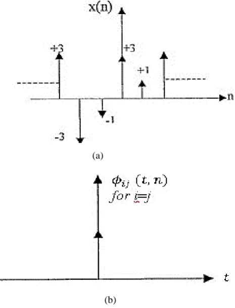
Suppose that the input signal is passed through a digital Low-Pass Filter (LPF), then, the output of the digital filter is applied to the adaptive system as shown in Fig. 1. To show the effect of the digital low pass filter on the adaptation process, let us discuss the difference between the input and the output signals of the digital filter. The input to the digital filter is shown in Fig. 2(a), where Fig. 2(b) shows the autocorrelation , where , with , . It can be observed from Fig. 2 that the input signal is an impulse signal at each instant and is correlated with itself only and it is never correlated with other impulses. The output of the digital low pass filter is also a random signal as shown in Fig. 3.(a)
(b)
Fig 2: The input signal and its autocorrelation, (a)the input signal to the digital LPF, (b) the autocorrelation of the input signal where
, with ,
[image:3.595.58.279.72.201.2].
Fig 3: The output of the digital low pass filter.
[image:3.595.313.546.369.588.2]Fig 4: The power spectral density of the input signal x(n)
It is seen from the demonstration of the LMS convergence that the algorithm convergence time is determined as,
(16)
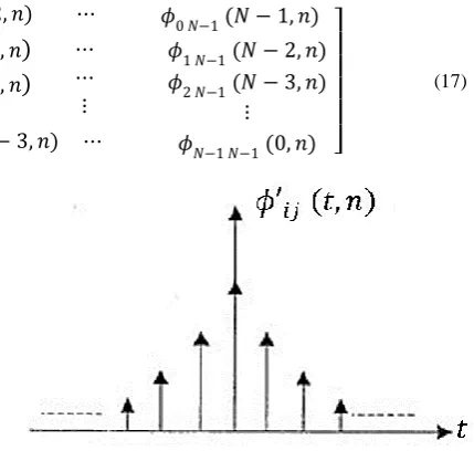
where , and are the minimum and maximum eigenvalues of the autocorrelation matrix respectively. The ratio of the maximum to minimum eigenvalue is called the eigenvalue disparity and determines the speed of convergence. The matrix is given as
(17)
where , with ,
. It is seen from (16) that the convergence time is inversely proportional to and depends only on the nature of the input sequence . The physical interpretation of the eigenvalues of can be illustrated by comparing them with the spectrum of the input signal . It is a classical result of Toeplitz form theory that the eigenvalues are bounded by,
(18)
where is the power spectral density of the input or the Fourier transform of the autocorrelation function (elements of the matrix). As the order of the matrix, N, tends to infinity,
(19)
Given that the convergence time can be expressed as in (16), one can infer that the spectra that with the ratio of the maximum to minimum spectrum is large results in sluggish convergence. Spectra with an eigenvalue disparity near unity (i.e., flat spectra) lead to rapid convergence. The conjecture about such results is that large correlation among the input samples is related to a large eigenvalue disparity, which in turn decelerates the convergence of the adaptation process of the FIR filter.
Now, the effect of colored signal on the convergence speed of adaptation process will be shown. The autocorrelation function of the colored signal is shown in Fig. 5.
Fig 5: The autocorrelation of the colored signal .
From Fig. 5, it can be verified that the impulse is more correlated with itself and less with other impulses. The spectral density of the input signal can be obtained by computing the Fourier transform of the autocorrelation function (the elements of matrix) as shown in Fig. 6. So
that the eigenvalue disparity
[image:4.595.327.533.545.675.2]will be larger than the white signal. Therefore, the effect of the colored signal will result in slow convergence.
Fig 6: The power spectral density of the digital filter output .
5.2
The Evolutionary LMS Algorithm
(LMS-GA)
learning the adaptive FIR and IIR filters is proposed in this section which incorporates the quintessence and features of both algorithms.
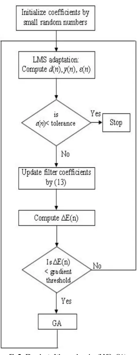
The essential principle of our novel learning algorithm is to combine the evolutionary idea of GA into the gradient-descent technique in order to give an organized random searching amid the gradient-descent calculations. The filter coefficients are represented as a chromosome with a list of real numbers in our proposed technique. The LMS algorithm is embedded in the mutation process of GA to discover the fastest shortcut path in adjusting the optimal solution through the learning process. Each time the LMS learning tool get caught in a local minimum, or the convergence of the LMS algorithm is slow (i.e., the gradient of the error is within a specific range), the GA is initiated by arbitrarily varying the estimated filter parameters values to obtain a new sets of filter coefficients. The proposed learning algorithm, namely, LMS-GA, chooses the filter among the new filters and the first one with the smallest MSE (best fitness value) as the new candidate to the next evolution. The above process will be done more and more if the convergence speed is detected to be sluggish at uniform intervals or the LMS algorithm stuck in one more local minimum. In the suggested learning technique, the parameters of the filter are varied during each evolution according to,
(20)
where is the permissible offset range for each evolution, m is the offsprings number produced in the evolutions, denotes the i-th offsprings that are produced by the parents filter , and [-1, +1] is a random number. To pick the optimum filter to be the next candidate amongst the sets of new offsprings in the course of each evolution, the MSE is calculated for each new filter ( , ) by (15) for block of time . The filter with the smallest MSE will be selected as the next candidate for the subsequent phase of learning process. The behavior of the new proposed LMS-GA is represented by the flowchart shown in Fig. 7. The ΔE(n) in the flowchart of Fig. 7 is the error gradient and defined as
where is the window size for estimation of
The computational complexity of the LMS algorithm of the FIR filter for the case of the white input signal is found to be (2 multiplication per iteration, where is the length of the FIR filter. While the computational complexity required for the IIR filter is equal to where is the backward length and is the forward length of the IIR filter for the same order of both FIR and IIR filters (i.e.,
). The computational complexity of the LMS algorithm of the FIR filter with colored the nput signal is given as
, where is the length of the digital LPF.
6.
NUMERICAL RESULTS
Consider 4-Tap adaptive FIR filter in channel equalization task and as a plant model for the purpose of system identification,
(21)
The basic idea of the system identification using adaptive FIR filtering depends on matching the coefficients of the adaptive filter to that of the plant. The convergence factor regulates the adaptation stability and convergence speed. The results of applying the standard LMS algorithm on adaptive FIR filter
to identify the parameters of (22) with different values of are shown in Table 1.
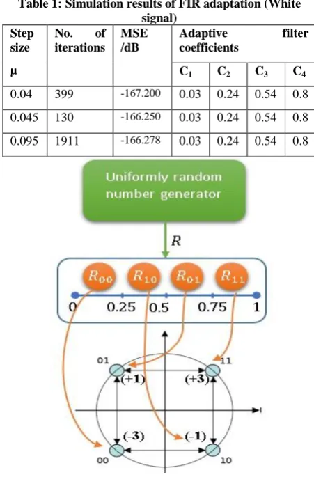
[image:5.595.318.542.169.748.2]A special class of input signal is generated to train the weights of the adaptive FIR filter, it consists of four level values (3, -1, +-1, and +3) and governed by a uniformly generated random input as shown in Fig. 8, e.g., if the random number is , i.e., it is in the range [0, 0.25], then , the same for other values of .
Table 1: Simulation results of FIR adaptation (White signal)
Step size
µ
No. of iterations
MSE /dB
Adaptive filter coefficients
C1 C2 C3 C4
0.04 399 -167.200 0.03 0.24 0.54 0.8
0.045 130 -166.250 0.03 0.24 0.54 0.8
0.095 1911 -166.278 0.03 0.24 0.54 0.8
Fig 8: Four levels input scheme used to train FIR and IIR adaptive filters.
[image:6.595.314.542.324.435.2]These four level input values generated using the scheme proposed in Fig. 8 are entered repeatedly into the input channel of Fig. 9 until a convergence is reached or maximum number of iterations are achieved.
Fig 9: System identification block diagram.
Table 2: Simulation results of FIR adaptation (Colored signal)
Step size µ
No. of iterations
MSE /dB
Adaptive filter coefficients C1 C2 C3 C4
0.9 2320 -135.591 0.03 0.24 0.54 0.8 3 358 -163.131 0.03 0.24 0.54 0.8 4 362 -173.604 0.03 0.24 0.54 0.8
Concerning the adaptive IIR filter, the error surface is generally a multi-modal against filter parameters. The adaptation techniques for the case of adaptive IIR filter can easily get stuck at a local minimum and escape away from the global minimum. Some of the adaptive IIR filter coefficients will be matched with that of the plant and the other will be constant at certain values, which means that these coefficients are stuck at local minima. The following 1st order transfer function is used to represent the plant,
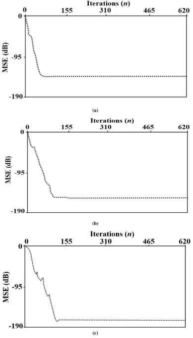
(22) The results of the system identification using IIR adaptive filtering are shown in Table 3. As can be seen, that the best value of was found to be 0.06 with mean square error of -143.939 dB. The IIR error surface here is a special case as it is an uni-modal (local minimum does not exists) and having a global optimum only. However, the practical problem still exists here which is the pole of the adaptive filter may move outside of the unit circle resulting in an unstable system. To solve this problem, a certain criterion is used, it states when the magnitude of the pole exceeds unity, its magnitude is limited to be less than one. The learning curves for different values of are shown in Fig. 10.
Table 3: Simulation of adaptive IIR filter (white signal) Step size
µ
No. of iterations
MSE /dB Adaptive filter coefficients
a b
0.04 142 -157.373 -0.2 0.6
0.06 63 -143.939 -0.2 0.6
0.1 134 -174.030 -0.2 0.6
Table 1 demonstrates the optimum value of that corresponds to less number of iterations which is found to be (0.045). For the case of the coloured input signal, the same input produced using the scheme of Fig. 8 is applied on the input channel of Fig. 1, it can be concluded that the spectra with the ratio of the maximum to minimum spectrum is large results in sluggish convergence. Spectra with an eigenvalue disparity near unity (i.e., flat spectra) lead to rapid convergence. The digital filter of Fig. 1 used in this simulation is of 8-Tap FIR LPF type given as,
While the plant dynamics is given in (22). Different ’s have been used in coloured input signal case study with the results given in Table 2. It is noted that the optimum value of that corresponds to the less number of iterations is found to be 3.The best value of is found with MSE of -163.131dB.
[image:6.595.57.281.500.649.2](a)
(b)
[image:7.595.111.501.73.757.2](c)
Table 4: Simulation results of both standard LMS and LMS-GA algorithms
Standard LMS algorithm with optimum µ
LMS-GA
with optimum µ
No. of iterations 130 336
MSE (dB) -166.250 -173.604
Fi
lter
Co
efficie
n
ts
C1 0.03 0.03
C2 0.24 0.24
C3 0.54 0.54
C4 0.8 0.8
The proposed LMS-GA learning tool is exploited to learn an adaptive IIR filter to recover the performance of the gradient descent technique (e.g., the LMS algorithm) with multi-modal error surface. To compare the new LMS-GA learning tool with the standard LMS algorithm, the window size δ must be determined for estimation of ∆E and the Gradient Threshold (GT), these can be calculated from the learning curve of the pure LMS algorithm as follows, window size τ is calculated as being the number of iterations between the first iteration and the iteration at which the learning curve fluctuate with a small variations. GT is calculated by determining the maximum and minimum values of these fluctuations. Now, GT can be determined as, GT=(max.swing-min.swing)/ δ. If these two parameters are calculated, one can apply the procedure of the new learning algorithm of Fig. 7 on adaptive IIR filter of a unimodal error surface as in (23). It can be concluded that the new learning algorithm will converge to the same MSE (the same MSE the pure LMS reached to it) but with a fewer number of iterations as shown in Fig. 11.
Fig 11: The convergence performance of the LMS-GA tool for adaptive IIR filter.
7.
CONCLUSIONS
In this work, adaptive algorithms are adopted to learn the parameters of the digital FIR and IIR filters such that the error signal is minimized. These algorithms are the standard LMS algorithm and the LMS-GA one. The numerical instabilities inherent in other adaptive techniques do not exist in the standard LMS algorithm. Moreover, prior information of the signal statistics is not required, i.e., the autocorrelation and cross-correlation matrices. The LMS algorithm produces only estimated adaptive filter coefficients. These estimated coefficients match that of the plant progressively through the
time as the coefficients are changed and the adaptive filter learns the signal characteristics, then identify the underlying plant. Due to the multimodality of the error surface of adaptive IIR filters, a new learning algorithm, namely, LMS-GA is proposed in this paper which integrates the genetic searching methodology LMS algorithm and speeds up the adaptation procedure and offers universal searching ability. Besides, the LMS-GA preserved the characteristics and the simplicity of the standard LMS learning algorithm and it entails comparatively fewer computations and had a fast convergence rate as compared to the standard GA. The numerical simulations evidently elucidated that the LMS-GA outperforms the standard LMS in terms of the capability to determine the global optimum solution and the faster convergence rate to this solution.
8.
REFERENCES
[1] S. D. S. Bernard Widrow, 1985. Adaptive Signal Processing. Prentice-Hall.
[2] J. C. S. and J. V. J. Gerardo Avalos. 2011. Applications of Adaptive Filtering. in Adaptive Filtering Applications, Lino Garcia Morales, Ed. InTech, pp. 1–20.
[3] M. Shams Esfand Abadi, H. Mesgarani, and S. M. Khademiyan. 2017. The wavelet transform-domain LMS adaptive filter employing dynamic selection of subband-coefficients. Digit. Signal Process., vol. 69, pp. 94–105, 2017.
[4] C. Y. C. S.C. Ng, S.H. Leung. 1996. The Genetic Search Approach: A new Learning Algorithm for Adaptive IIR Filtering. IEEE Signal Process. Mag., vol. 13, no. 6, pp. 38–46.
[5] S. M. Kumpati S. Narendra. 1997. Neural Networks for System Identification. IFAC System Identification, Vol. 30, No. 11, pp. 735–742.
[6] D. R. Santosh Kumar Behera. 2014. System Identification Using Recurrent Neural Network. Int. J. Adv. Res. Electr. Electron. Instrum. Eng., Vol. 3, No. 3, pp. 8111–8117.
[7] H. Jaeger. 2003. Adaptive nonlinear system identification with echo state networks. Advances in Neural Information Processing Systems, pp. 593–600.
[8] W. Zhang. 2007. System Identification Based on a Generalized ADALINE Neural Network. American Control Conference (ACC), 2007, Vol. 11, No. 1, pp. 4792–4797.
[9] Ibraheem. Kasim Ibraheem. 2017. System Identification of Thermal Process using Elman Neural Networks with No Prior Knowledge of System Dynamics. Int. J. Comput. Appl., Vol. 161, No. 11, pp. 38–46.
[10] V. Katari, S. Malireddi, S. K. S. Bendapudi, and G. Panda. 2008. Adaptive nonlinear system identification using comprehensive learning PSO. 3rd International Symposium on Communications, Control and Signal Processing( ISCCSP), pp. 434–439.
[11] A. C. Sinha, Rashmi. 2017. Adaptive Filtering Via Wind Driven Optimization Technique. 3rd IEEE International Conference on Computational Intelligence and Communication Technolog (CICT), pp. 1–5.
[image:8.595.53.275.437.614.2]and Engineering Management (IEEM), Singapore, Singapore, pp. 752–755.
[13] J. Zhang and P. Xia. 2017. An improved PSO algorithm for parameter identification of nonlinear dynamic hysteretic models,” J. Sound Vib., vol. 389, pp. 153–167.
[14] A. Sarangi, S. K. Sarangi, M. Mukherjee, and S. P. Panigrahi. 2015. System identification by Crazy-cat swarm optimization. 2015 International Conference on Microwave, Optical and Communication Engineering (ICMOCE), pp. 439–442.
[15] K. K. A.-M. Thamer M. Jamel. 2012. Simple Variable Step Size LMS Algorithm for Adaptive Identification of IIR Filtering System. 5th International Conference on Communications, Computers and Applications (MIC-CCA), Istanbul, Turkey, pp. 23–28.
[16] S. A. Ghauri and M. F. Sohail. 2013. System identification using LMS, NLMS and RLS. Proceeding - IEEE Student Conference on Research and Development, (SCOReD), no. December, pp. 65–69.
[17] L. Lu and H. Zhao. 2015. A novel convex combination of LMS adaptive filter for system identification. 12th
International Conference on Signal Processing Proceedings (ICSP), Hangzhou, China pp. 225–229.
[18] R. Yu, Y. Song, and M. Nambiar. 2014. Fast system identification using prominent subspace LMS. Digit. Signal Process. A Rev. J., Vol. 27, No. 1, pp. 44–56,.
[19] F. Titel and K. Belarbi. 2013. Identification of Dynamic systems using a Genetic Algorithm-based Fuzzy Wavelet Neural Network approach,” in Proceedings of the 3rd International Conference on Systems and Control, 2013, pp. 6–11.
[20] Alyaa. A. AL-Husainy, Ibraheem Kasim Ibraheem. 2014. Application of an Evolutionary Optimization Technique to Routing in Mobile Wireless Networks Application of an Evolutionary Optimization Technique to Routing in Mobile Wireless Network. Int. J. Comput. Appl., Vol. 99, No. 7, pp. 24–31,.