Testing for a Change in Mean After
Changepoint Detection
Sean Jewell
∗Department of Statistics, University of Washington
Paul Fearnhead
Department of Mathematics and Statistics, Lancaster University
Daniela Witten
Departments of Statistics and Biostatistics, University of Washington
Abstract
While many methods are available to detect structural changes in a time series, few procedures are available to quantify the uncertainty of these estimates post-detection. In this work, we fill this gap by proposing a new framework to test the null hypothesis that there is no change in mean around an estimated changepoint. We further show that it is possible to efficiently carry out this framework in the case of changepoints estimated by binary segmentation, variants of binary segmentation,
`0 segmentation, or the fused lasso. Our setup allows us to condition on much smaller selection events than existing approaches, which yields higher powered tests. Our procedure leads to improved power in simulation and additional discov-eries in a dataset of chromosomal guanine-cytosine content. Our new changepoint inference procedures are freely available in the Rpackage ChangepointInference at https://jewellsean.github.io/changepoint-inference/.
Keywords: `0 optimization, binary segmentation, fused lasso, selective inference
∗Sean Jewell received funding from the Natural Sciences and Engineering Research Council of
Canada. This work was partially supported by Engineering and Physical Sciences Research Council Grant EP/N031938/1 to Paul Fearnhead, and NSF CAREER DMS-1252624, NIH grants DP5OD009145, R01DA047869, and R01EB026908, and a Simons Investigator Award in Mathematical Modeling of Liv-ing Systems to Daniela Witten.
1 Introduction
Detecting structural changes in a time series is a fundamental problem in statistics, with a variety of applications (Bai and Perron, 1998, 2003; Muggeo and Adelfio, 2010;
Schr¨oder and Fryzlewicz, 2013; Futschik et al., 2014; Xiao et al., 2019; Harchaoui and
L´evy-Leduc,2007;Hotz et al.,2013). A structural change refers to the phenomenon that
at certain (unknown) timepoints, the law of the data may change: that is, observations y1, . . . , yT are heterogeneous in the sense that y1, . . . , yτ ∼F, whereas yτ+1, . . . , yT ∼G,
for distribution functions F 6=G. In the presence of possible structural changes, it is of interest not only to estimate the times at which these changes occur — that is, the value of τ — but also to conduct statistical inference on the estimated changepoints.
In this paper, we consider the most common changepoint model
Yt=µt+t, t iid
∼N(0, σ2), t = 1, . . . , T, (1)
and assume thatµ1, . . . , µT is piecewise constant, in the sense thatµτj+1 =µτj+2 =. . .=
µτj+1, µτj+1 6= µτj+1+1, for j = 0, . . . , K −1, where 0 = τ0 < τ1 < . . . < τK < τK+1 =T,
and where τ1, . . . , τK represent the true changepoints. Changepoint detection refers to
the task of estimating the changepoint locations τ1, . . . , τK, and possibly the number
of changepoints K. A huge number of proposals for this task have been made in the literature, and can be roughly divided into two classes. One class of proposals iter-atively searches for one changepoint at a time (Vostrikova, 1981; Olshen et al., 2004;
Fryzlewicz et al., 2014; Badagi´an et al., 2015; Anastasiou and Fryzlewicz, 2019); the
canonical example of this approach is binary segmentation. Another class of propos-als involves simultaneously estimating all changepoints by solving a single optimization problem (Auger and Lawrence,1989;Jackson et al.,2005;Tibshirani et al.,2005;Niu and
Zhang, 2012;Killick et al., 2012; Haynes et al.,2017; Maidstone et al.,2017; Jewell and
Witten,2018;Fearnhead et al.,2019; Hocking et al.,2018;Jewell et al., 2019); examples
include `0 segmentation and the fused lasso. We review these approaches in Section2.
in extreme cases, this could include an estimated changepoint that is almost as far as T /2 observations from an actual changepoint.
In this paper, we consider testing the null hypothesis that there is no change in mean around an estimated changepoint. This is challenging since we must account for the estimation process when deriving the null distribution for a test statistic. A recent promising line of work was introduced by Hyun et al. (2016) and Hyun et al.
(2018), who develop valid tests that appropriately control for the estimation process in the cases where changepoints are estimated with the generalized lasso and with binary segmentation, respectively. They leverage recent results for selective inference in the regression setting (Fithian et al., 2014, 2015; Tibshirani et al., 2016; Lee et al., 2016;
Tian et al., 2018).
One disadvantage of the proposals of Hyun et al. (2016) and Hyun et al. (2018) is that, when defining p-values, they need to condition on much more information than is used to choose the null hypothesis that is tested. This is especially relevant sinceFithian
et al. (2014), Lee et al. (2016), and Liu et al. (2018) show that conditioning on extra
information leads to a reduction in power. Our contribution is to implement selective inference while conditioning on less information, and moreover to illustrate that selective inference techniques can be used when changepoints are detected via `0 segmentation.
Our empirical results show that both these advances lead to more powerful procedures for testing for the presence of changepoints. We develop this framework in detail for the change-in-mean model, but the general ideas can be applied more widely.
The rest of this paper is organized as follows. In Section 2, we review the relevant literature on changepoint detection and inference. In Section3, we introduce a framework for inference in changepoint detection problems, which allows us to test for a change in mean associated with a changepoint estimated on the same dataset. In Sections 4 and
5, we develop efficient algorithms that allow us to instantiate this framework in the special cases of binary segmentation (Vostrikova, 1981) and its variants (Olshen et al.,
2004;Fryzlewicz et al.,2014), and`0 segmentation (Killick et al., 2012;Maidstone et al.,
2017); the case of the fused lasso (Tibshirani et al.,2016) is straightforward and addressed in the Supplementary Materials. Our framework is an improvement over the existing approaches for inference on the changepoints estimated using binary segmentation and its variants and the fused lasso; it is completely new in the case of `0 segmentation.
In Section 6, we examine the performance of our proposal, and compare it to some recent proposals from the literature, in a simulation study. In Section 7, we show that our procedure leads to additional discoveries versus existing methods on a dataset of chromosomal guanine-cytosine (G-C) content. Extensions are in Section 8, and some additional details are deferred to the Supplementary Materials.
Our new changepoint inference procedures are freely available in the R package
ChangepointInference. Code and data to produce all figures is available at
2 Background
2.1 Changepoint detection algorithms
2.1.1 Binary segmentation and its variants
The binary segmentation proposal of Vostrikova (1981) and its variants (Olshen et al.,
2004; Fryzlewicz et al., 2014) search for changepoints by solving a sequence of local
optimization problems. For the change-in-mean problem, these use the cumulative sum (CUSUM) statistic
g(s,τ,e)> y:=
s 1 1 |e−τ|+ 1 |τ+1−s|
(¯y(τ+1):e−y¯s:τ), (2)
defined through a contrastg(s,τ,e) ∈RT, which summarizes the evidence for a change atτ
in the data ys:e := (ys, . . . , ye) by the difference in the empirical mean of the data before
and after τ (normalized to have the same variance for all τ).
In binary segmentation (Vostrikova, 1981), the set of estimated changepoints is sim-ply the set of local CUSUM maximizers: the first estimated changepoint maximizes the CUSUM statistic over all possible locations, ˆτ1 = argmax
τ∈[1:(T−1)]
n
|g>(1,τ,T)y|o. Subsequent changepoints are estimated at the location that maximizes the CUSUM statistic when we consider regions of the data between previously estimated changepoints. For example, the second estimated changepoint is ˆτ2 = argmax
τ∈[1:(T−1)]\τˆ1 n
|g>
(1,τ,ˆτ1)y|1(1≤τ <ˆτ1)+|g
>
(ˆτ1,τ,T)y|1(ˆτ1<τ <T) o
.
We continue in this manner until a stopping criterion is met. Variants of this procedure have been proposed to improve performance (Olshen et al.,2004;Fryzlewicz et al.,2014).
2.1.2 Simultaneous estimation of changepoints
As an alternative to sequentially estimating changepoints, we can simultaneously esti-mate all changepoints by minimizing a penalized cost that trades off fit to the data against the number of changepoints (Killick et al., 2012; Maidstone et al., 2017), i.e.
minimize
0=τ0<τ1<···<τK<τK+1=T,
u0,u1,...,uK,K
( 1 2 K X k=0 ˆ τk+1 X
t=ˆτk+1
(yt−uk)2+λK
)
. (3)
This is equivalent to solving an `0 penalized regression problem
minimize
µ∈RT
( 1 2 T X t=1
(yt−µt)2+λ T
X
t=2
1(µt6=µt−1) )
in the sense that the vector ˆµ that solves (4) is piecewise constant with breakpoints at ˆ
τ1, . . . ,τˆKˆ, where ˆτ1, . . . ,τˆKˆ are the changepoints that solve (3). Here, λ is a tuning
parameter that specifies the improvement in fit to the data needed to add an additional changepoint.
Replacing the `0 penalty in (4) with an `1 penalty leads to the well-studied trend
filtering or fused lasso optimization problem (Rudin et al.,1992;Tibshirani et al.,2005),
minimize
µ∈RT
(
1 2
T
X
t=1
(yt−µt)2+λ T
X
t=2
|µt−µt−1|
)
. (5)
2.2 Existing methods for inference on changepoints
Suppose we wish to quantify the evidence for a set of estimated changepoints ˆτ1, . . . ,τˆKˆ.
We could naively apply a standardz-test for the difference in mean around each estimated changepoint. However, this procedure is fundamentally flawed since the same data is used to estimate the changepoints and thus to choose the hypothesis tests that we perform. Therefore, the z-statistic is not normally distributed under the null hypothesis. In the linear regression setting, Tibshirani et al.(2016) and Lee et al. (2016) have shown that it is possible to select and test hypotheses based on the same set of data, provided that we condition on the output of the hypothesis selection procedure.
Hyun et al. (2016) and Hyun et al. (2018) extend these ideas to the changepoint
detection setting. For each changepoint ˆτj estimated using either binary segmentation,
its variants, or the fused lasso, Hyun et al. (2018) propose to test whether there is a change in mean around ˆτj. They construct the test statistic ˆdjν>Y, where ˆdj is the sign
of the estimated change in mean at ˆτj, andν is a T-vector of contrasts, defined as
νt =
0 if t≤τˆj−1 ort >τˆj+1, 1
ˆ
τj−ˆτj−1 if ˆτj−1 < t≤τˆj,
− 1
ˆ
τj+1−ˆτj if ˆτj < t≤τˆj+1,
(6)
and consider the null hypothesis H0 : ˆdjν>µ = 0 versus the one-sided alternative H1 :
ˆ
djν>µ >0. Since both ˆdj andν are functions of the estimated changepoints themselves,
it is clear that valid inference requires somehow conditioning on the estimation process in the spirit of Tibshirani et al. (2016) and Lee et al. (2016). Define M(y) to be the set of changepoints estimated from the data y, i.e., M(y) = {τˆ1, . . . ,τˆKˆ}. Then, it is
tempting to define the p-value as
PrH0
ˆ
djν>Y ≥dˆjν>y| M(Y) =M(y)
. (7)
However, (7) is not immediately amenable to the selective inference framework proposed
be polyhedral; i.e., the conditioning set can be written as{y:Ay≤b}for a matrixAand vectorb. Thus, in the case of binary segmentation, Hyun et al.(2018) condition on three additional quantities: (i) the order in which the estimated changepoints enter the model,
O(Y) = O(y); (ii) the sign of the change in mean due to the estimated changepoints, ∆(Y) = ∆(y) = {dˆ1, . . . ,dˆK}; (iii) Π⊥νY = Π⊥νy, where Π⊥ν = I − νν>/||ν||22 is the
orthogonal projection matrix onto the subspace that is orthogonal to ν. Conditions (i) and (ii) ensure that the conditioning set is polyhedral, whereas condition (iii) ensures that the test statistic is a pivot. This leads to the p-value
PrH0
ˆ
djν>Y ≥dˆjν>y| M(Y) =M(y),O(Y) =O(y),∆(Y) = ∆(y),Π⊥νY = Π⊥νy
, (8)
which can be easily computed because the conditional distribution of ˆdjν>Y is a Gaussian
truncated to an interval, which is computationally tractable. For slightly different condi-tioning sets, Hyun et al. (2018) show similar results for variants of binary segmentation and for the fused lasso.
Importantly, Hyun et al. (2018) choose the conditioning set in (8) for computational reasons: there is no clear statistical motivation for conditioning on O(Y) = O(y) and ∆(Y) = ∆(y). Furthermore, it might be possible to account for the fact that change-points are estimated from the data without conditioning on the full set M(Y) = M(y). In fact,Fithian et al. (2014) argue that when conducting selective inference, it is better to condition on a smaller set, since conditioning on more information reduces the Fisher information that remains in the conditional distribution of the data.
For this reason, in the regression setting, some recent proposals seek to reduce the size of the conditioning set. Lee et al.(2016) propose to condition on just the selected model, rather than on the selected model and the corresponding coefficient signs, by considering all possible configurations of the signs of the estimated coefficients. Unfortunately, this comes at a significant computational cost. Continuing in this vein, Liu et al. (2018) partition the selected variables into high value and low value subsets, and then condition on the former and the variable of interest.
In this paper, we develop new insights that allow us to test the null hypothesis that there is no change in mean at an estimated changepoint, without restriction to the polyhedral conditioning sets pursued byHyun et al. (2018). This means that we do not need to use the full conditioning set in (8), and, in turn, leads to higher-powered tests. Additionally, since we do not need to condition on ∆(Y) = ∆(y), we are able to consider two-sided tests of
H0 :ν>µ= 0 versus H1 :ν>µ6= 0, (9)
rather than the one-sided tests considered by Hyun et al.(2018).
1995; Benjamini et al., 2001; Barber et al., 2015; Candes et al., 2018). However, these alternatives are not suitable for the changepoint setting in the following sense. Often we do not want to know if a true changepoint is exactly at ˆτj, but rather whether there is a
true changepoint near τˆj; that is, we are willing to accept small estimation errors in the
location of a changepoint. By suitable choice of ν in (9), we can test whether there is a change in mean near ˆτj, wherenear can be defined appropriately for a given application.
It is possible that application of, for example, knockoffs (Barber et al., 2015; Candes
et al., 2018) would enable us to control the false discovery rate for the null hypotheses
that the changes in mean are precisely at ˆτ1, . . . ,τˆKˆ. However, our experience with such
methods is that they have almost no power to detect small to moderate changes in the mean, due to the large uncertainty in the precise location of the change.
2.3 Toy example illustrating the cost of conditioning
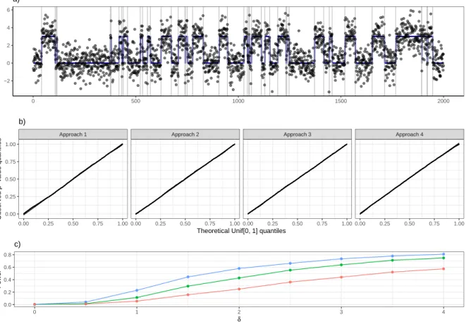
In this section, we demonstrate that the power of a test of (9) critically depends on the size of the conditioning set. In Figure 1, we consider two choices for the conditioning set. In panel a), we condition on M(Y) = M(y),O(Y) = O(y),∆(Y) = ∆(y), and Π⊥
νY = Π⊥νy (which is essentially the test proposed by Hyun et al. (2018)). In panel
b) we condition on just M(Y) = M(y) and Π⊥
νY = Π⊥νy. Observed data (grey points)
are simulated according to (1) with the true underlying mean displayed in blue. 19-step binary segmentation is used to estimate changepoints, which are displayed as vertical lines, and are colored based on whether the associated p-value is less than 0.05 (blue) or greater than 0.05 (red). In this example, conditioning on a smaller set allows us to reject the null hypothesis when it is false more often (i.e., we obtain five additional true positives), without inflating the number of false positives.
With this toy example in mind, we turn to our proposal in the following section. It does not require polyhedral conditioning sets, and thus allows us to condition on much smaller sets than previously possible.
3 Two new tests with smaller conditioning sets
In this section, we consider testing a null hypothesis of the form (9) using a much smaller conditioning set than used by Hyun et al. (2018). Our approach is similar in spirit to the “general recipe” proposed in Section 6 ofLiu et al.(2018). We consider two possible forms of the contrast vector ν in Sections 3.1 and 3.2.
3.1 A test of no change in mean between neighboring changepoints
estimated changepoints, M(y) ={τˆ1, . . . ,τˆKˆ}. Thus, we define the p-value
p≡PrH0 |ν>Y| ≥ |ν>y| | M(Y) = M(y),Π⊥νY = Π⊥νy
. (10)
As in Hyun et al. (2018), we condition on Π⊥
νY = Π⊥νyfor technical reasons; see Fithian
et al. (2014) for additional discussion. Roughly speaking, (10) asks: “Out of all data
sets yielding this particular set of changepoints, what is the probability, under the null that there is no changepoint at this location, that the difference in mean between the segments on either side of ˆτj is as large as what is observed?”
Our next result reveals that computing (10) involves a univariate truncated normal distribution.
Theorem 1 The p-value in (10) is equal to
p=Pr |φ| ≥ |ν>y| | M(y0(φ)) = M(y), (11)
where φ∼N(0,kνk2σ2) and where
y0(φ) = y− νν>y ||ν||2 2
+ νφ
||ν||2 2
. (12)
In light of Theorem 1, to evaluate (10) we must simply characterize the set
S ={φ :M(y0(φ)) =M(y)}; (13)
as we will see in Section3.3, this is the set of perturbations ofy that result in no change to the estimated changepoints. In Sections 4 and 5, we do exactly this in the case of binary and `0 segmentation, respectively. We discuss the fused lasso in Section D of the
Supplementary Materials.
3.2 A test of no change in mean within a fixed window size
We now consider testing the null hypothesis that there is no change in mean in a window h >0 around thejth estimated changepoint,
H0 :µτˆj−h+1 =. . .=µτˆj =. . .=µˆτj+h. (14)
This is a special case of (9) forν defined as
νt =
0 if t≤τˆj−h or t >ˆτj +h, 1
h if ˆτj −h < t≤τˆj,
−1
h if ˆτj < t≤τˆj +h.
When considering this null hypothesis, it makes sense to condition only on the jth estimated changepoint, leading to a p-value defined as
p≡PrH0 |ν>Y| ≥ |ν>y| |ˆτj ∈ M(Y),Π⊥νY = Π⊥νy
, (16)
where once again, we condition on Π⊥νY = Π⊥νy for technical reasons. Roughly speaking, (16) asks: “Out of all data sets yielding a changepoint at ˆτj, what is the probability,
under the null that there is no changepoint at this location, that the difference in mean within a fixed window of ˆτj is as large as what is observed?”
The p-values in (16) and (10) are calculated for slightly different null hypotheses: the null for (16) is that there is no changepoint within a distance h of the estimated changepoint, ˆτj. By contrast, (10) tests for no change in mean between the estimated
changepoints immediately before and after ˆτj. Furthermore, (16) conditions on less
information. We believe that in many applications, the null hypothesis assumed by (16) is more natural and informative since it allows a practitioner to specify how accurately they want to detect changepoint locations, and it avoids rejecting the null due to changes that are arbitrarily far away from ˆτj. Moreover, the ability to condition on less information
intuitively should lead to higher power. If required, the ideas used to calculate (16) could also be applied to test for the null hypothesis assumed by (10), while conditioning on less information. We further investigate these issues in Sections 6 and 8.1.
Theorem 1can be extended to show that (16) is equal to
p= Pr |φ| ≥ |ν>y| |τˆj ∈ M(y0(φ))
, (17)
where φ ∼ N(0,kνk2σ2), and where y0(φ) was defined in (12). Thus, computing the
p-value requires characterizing the set
S ={φ : ˆτj ∈ M(y0(φ))}; (18)
this is the set of perturbations of y that result in estimating a changepoint at ˆτj.
We show in Sections 4and 5that S can be efficiently characterized for binary and`0
segmentation. We discuss the fused lasso in Section D of the Supplementary Materials.
3.3 Intuition for y0(φ) and S
To gain intuition for y0(φ) in (12), we consider ν defined in (6). We see that
yt0(φ)≡
yt if t≤τˆj−1 ort >τˆj+1,
yt+ φ−ν
>y
1+τjˆˆ−ˆτj−1
τj+1−ˆτj
if ˆτj−1 < t≤τˆj,
yt− φ−ν
>y
1+τjˆˆ+1−τjˆ
τj−τjˆ−1
if ˆτj < t≤τˆj+1.
Thus, y0t(φ) is equal to yt for t ≤ τˆj−1 or t > τˆj+1, and otherwise equals the observed
data perturbed by a function of φ around ˆτj. In other words, we can view y0(φ) as a
perturbation of the observed datay by a quantity proportional to φ−ν>y, within some
window of ˆτj. Furthermore, S ={φ :M(y0(φ)) =M(y)}is the set of such perturbations
that do not affect the set of estimated changepoints.
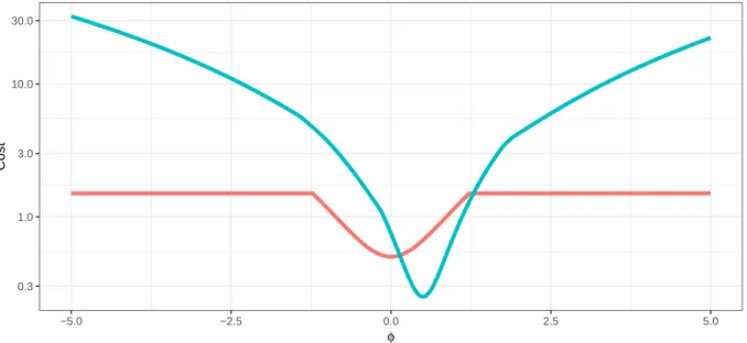
Figure 2 illustrates the intuition behind y0(φ) in a simulated example with a change
in mean at the 100th position, and where φ = ν>y = −1. In panel a), the observed data are displayed. Here, 1-step binary segmentation estimates ˆτ1 = 100. In panel b),
the observed data are perturbed using φ = 0 so that 1-step binary segmentation no longer estimates a changepoint at the 100th position. Conversely, in panel c), the data are perturbed using φ = −2 to exaggerate the change at timepoint 100; 1-step binary segmentation again estimates a changepoint at the 100th position. Hence, for 1-step binary segmentation, −1 and −2 are inS ={φ:M(y0(φ)) = M(y)}, but 0 is not.
In Sections 4 and 5, and in Section D of the Supplementary Materials, we develop procedures to characterizeS in the cases of binary segmentation,`0segmentation, and the
fused lasso, respectively. Here, the procedure from Section 4gives S ={φ :M(y0(φ)) =
M(y)}= (−∞,−0.2)∪(0.2,∞); see panel d) of Figure 2.
4 Efficient characterization of (13) and (18) for binary segmentation
We now turn our attention to computing the set (13) for k-step binary segmentation; (18) is detailed in Section B.3 of the Supplementary Materials. Extensions to variants of binary segmentation proposed in Olshen et al.(2004) and Fryzlewicz et al.(2014) are straightforward and, for brevity, are not included.
We begin by paraphrasing Proposition 1 of Hyun et al. (2018).
Proposition 1 (Proposition 1 of Hyun et al. (2018)) The set of y for which k
-step binary segmentation yields a given set of estimated changepoints, orders, and signs is polyhedral, and takes the form {y:Γy ≤0} for a k(2T −k−3)×T matrix Γ, which is a function of the estimated changepoints, orders, and signs.
We will now make use of this result in a new proposition. Recall from Section 2.2 that
M(y), O(y), and ∆(y) are defined as the set of estimated changepoints, orders, and signs.
Proposition 2 The set {φ :M(y0(φ)) = m,O(y0(φ)) = o,∆(y0(φ)) = d} is an interval.
Furthermore, the set S defined in (13) can be written as the union of such intervals,
S ={φ:M(y0(φ)) =M(y)}=
N0
[
i=−N
where N0+N + 1 is the number of elements in the set
I :={(o, d) :∃α∈R such thato =O(y0(α)), d= ∆(y0(α)),M(y) = M(y0(α))}. (21)
That is, I is the set of possible orders and signs of the changepoints that can be obtained via a perturbation of y that yields changepoints M(y).
Importantly, the set I has far fewer than 2kk! elements, which is the total number of
possible orders and signs for the k changepoints. The reason for the unconventional indexing in Proposition 2 will soon become apparent. Proposition 3 guarantees that Proposition 2is of practical use.
Proposition 3 SNi=0−N(ai, ai+1) defined in (20) can be efficiently computed.
Proposition 3 follows from a simple argument that we outline here. We first run k-step binary segmentation on the datayto obtain estimated changepointsM(y), ordersO(y), and signs ∆(y). We then apply the first statement in Proposition 2 with m = M(y), o=O(y), and d= ∆(y) to identify the interval [a0, a1]. By construction, [a0, a1]⊂ S.
Next, for some small positive value ofη, we apply the first statement in Proposition2
with m = M(y0(a
1 +η)), o = O(y0(a1 +η)), and d = ∆(y0(a1 +η)) to identify the
interval [a1, a2]. (If the left endpoint of this interval does not equal a1, then we must
repeat with a smaller value of η.) We then check whether M(y0(a1 +η)) = M(y); if
so, then [a1, a2] ⊂ S, and if not, then [a1, a2] 6⊂ S. Next, we apply the first statement
of Proposition 2 with m =M(y0(a
2+η)), o = O(y0(a2+η)), and d = ∆(y0(a2+η)) to
identify the interval [a2, a3]. We then determine whether [a2, a3] ⊂ S. We continue in
this way until we reach an interval containing ∞. We then repeat this process in the other direction, applying the first statement of Proposition 2 with m =M(y0(a
0 −η)),
o=O(y0(a0−η)), and d= ∆(y0(a0−η)), and determining whether the resulting interval
[a−1, a0] belongs to S, until eventually we arrive at an interval containing−∞.
Proposition4shows that this procedure can be stopped early in order to substantially reduce computational costs, and obtain conservative p-values.
Proposition 4 Let S˜ be defined as the set
˜
S = (−∞, a−r)∪
( r0
[
i=−r
(ai, ai+1)
)
∪(ar0+1,∞),
for some r < N and r0 < N0, and for a−r ≤ −|ν>y| andar0+1 ≥ |ν>y|. Then the p-value
obtained by conditioning on {φ∈S}˜ is greater than the p-value obtained by conditioning on {φ ∈ S}, i.e.,
SectionBof the Supplementary Materials contains proofs of Propositions 2and 4. In that section, we also show that Propositions2and3can be easily modified to characterize (18). Section D of the Supplementary Materials contains a straightforward modification of this procedure to characterize (13) and (18) in the case of the fused lasso.
5 Efficient characterization of (13) and (18) for `0 segmentation
In this section, we develop efficient algorithms to analytically characterize (13) for the `0 segmentation problem (4) with a fixed value of λ; Section C.2 of the Supplementary
Materials considersSin the case of (18). In particular, we wish to determine all values of φ such thatφ ∈ S, without checking each value of φ individually. Roughly speaking, we show that it is possible to write (13) in terms of the cost to segment the perturbed data y0(φ). To compute the necessary cost functions, we derive recursions that look similar
to those in Rigaill (2015) and Maidstone et al. (2017). However these recursions are for functions of two variables, rather than one, which requires fundamentally different techniques to avoid a computational cost that increases exponentially in h.
Let ˆK denote the number of estimated changepoints resulting from `0 segmentation
(4) on the original data y with fixed tuning parameter value λ, and let ˆτ1 < . . . < τˆKˆ
denote the positions of those estimated changepoints; for notational convenience, let ˆ
τ0 ≡0 and ˆτK+1ˆ ≡T. Recall the definition ofy0(φ) in (12) and the definition ofν in (6).
For a given value of φ, M(y0(φ)) = M(y) if and only if the cost of `0 segmentation of
the data y0(φ) with the changepoints restricted to occur at ˆτ
1, . . . ,τˆKˆ,
C(φ) = min
u0,u1,...,uKˆ
1 2
ˆ K
X
k=0 ˆ τk
X
t=ˆτk+1
(yt0(φ)−uk)2+λKˆ
, (22)
is no greater than the cost of `0 segmentation of y0(φ),
C0(φ) = min
0=τ0<τ1<···<τK<τK+1=T,
u0,u1,...,uK,K
(
1 2
K
X
k=0 τk+1 X
t=τk+1
(yt0(φ)−uk)2+λK
)
. (23)
In other words, S ={φ:C(φ)≤C0(φ)}. The following result will prove useful.
Proposition 5 C(φ) = C(φ0) for all φ and φ0.
Proposition 5 follows from the fact that from (12) and (6), y0(φ) is equal to y t for
t≤τˆj−1ort >τˆj+1, adds a constant that depends onφto all data points for ˆτj−1 < t≤τˆj,
and subtracts a constant from all data points for ˆτj < t≤τˆj+1. Therefore, by inspection
Applying Proposition 5, we see that S = {φ : C(ν>y) ≤ C0(φ)}. Furthermore, C(ν>y) is easy to calculate, by inspection of (22) (recall from (12) that y0(ν>y) = y).
Hence, we simply need an efficient way to calculateC0(φ), i.e., to perform`
0 segmentation
on the perturbed data. In the interest of computational tractability, we need a single procedure that works for all values ofφsimultaneously, rather than (for instance) having to repeat the procedure for values of φ on a fine grid.
We note that C0(φ) can be decomposed into the cost of segmenting the data y0(φ) with a changepoint at ˆτj,
Cˆτ0j(φ) = minu
n
Cost(y01:ˆτj(φ);u)
o
+ min
u0
n
Cost(yT0:(ˆτj+1)(φ);u
0)o+λ, (24)
and the cost of segmenting the data y0(φ) without a changepoint at ˆτj,
C¬ˆ0τj(φ) = min
u
n
Cost(y1:ˆ0 τj(φ);u) + Cost(y0T:(ˆτj+1)(φ);u)o, (25)
where Cost(y0
1:ˆτj(φ);u) is the cost of segmenting y
0
1:ˆτj(φ) with µτˆj = u. Combining (24)
and (25), we have
C0(φ) = minnCˆτ0j(φ), C¬ˆ0τj(φ)o. (26)
Next, we will show that it is possible to analytically calculate Cost(y0
1:ˆτj(φ);u) as a
function of the perturbation, φ, and the mean at the ˆτjth timepoint, u. A similar
approach can be used to compute Cost(yT0:(ˆτj+1)(φ);u).
5.1 Analytic computation of Cost(y0
1:ˆτj(φ);u)
We first note that Cost(y1:s;u), the cost of segmentingy1:swithµs =u, can be efficiently
computed (Rigaill,2015;Maidstone et al.,2017). The cost at the first timepoint is simply Cost(y1;u) = 12(y1 −u)2. For any s >1 and for all u,
Cost(y1:s;u) = min
n
Cost(y1:(s−1);u),min u0
Cost(y1:(s−1);u0) +λ
o
+ 1
2(ys−u)
2. (27)
For each u, this recursion encapsulates two possibilities: (i) there is no changepoint at the (s− 1)st timepoint, and the optimal cost is equal to the previous cost plus the cost of a new data point, Cost(y1:(s−1);u) + 12(ys −u)2; (ii) there is a changepoint at
the (s−1)st timepoint, and the optimal cost is equal to the optimal cost of segment-ing up to s−1 plus the penalty for adding a changepoint at s−1 plus the cost of a new data point, min
u0
Cost(y1:(s−1);u0) +λ+ 12(ys−u)2. The resulting cost functions
blush, the recursion appears to be intractable due to the fact that, naively, Cost(y1:s;u)
needs to updated for each value ofu∈R. However, amazingly,Rigaill (2015) and
Maid-stone et al.(2017) show that these updates can be performed by efficiently manipulating
piecewise quadratic functions ofu, without needing to explicitly consider individual val-ues of u, using a procedure that they call functional pruning.
It turns out that many of the computations made in the recursion (27) can be reused in the calculation of Cost(y1:ˆ0 τj(φ);u). In particular, we note that from (12) and (6), y0
s(φ) = ys for all s /∈ {τˆj−1 + 1, . . . ,τˆj+1}, and therefore, Cost(y1:ˆ0 τj−1(φ);u) =
Cost(y1:ˆτj−1;u). As a result, we only require a new algorithm to efficiently compute
Cost(y01:(ˆτj−1+1)(φ);u), . . . ,Cost(y01:ˆτj(φ);u). However, since these cost functions are piece-wise quadratic of two variables, developing functional pruning recursions similar to the one-dimensional recursions of (27) is fundamentally more difficult. Nonetheless, in The-orem 2 we show that Cost(y0
1:s(φ);u) for s = ˆτj−1+ 1, . . . ,τˆj is the pointwise minimum
over a set Cs that can be efficiently computed.
Theorem 2 For τˆj−1 < s≤τˆj,
Cost(y1:s0 (φ);u) = min
f∈Cs
f(u, φ),
where {f(u, φ)}f∈Cs is a collection of s −τˆj−1 + 1 piecewise quadratic functions of u
and φ constructed recursively from τˆj−1 + 1 to s, and where Cτˆj−1 = {Cost(y1:ˆτj−1;u)}.
Furthermore, the set Cτˆj can be computed in O((ˆτj −τˆj−1)
2) operations.
Theorem 2 is proven in SectionC.1 of the Supplementary Materials. Timing results are in Section C.4 of the Supplementary Materials.
5.2 Computing C0(φ) based on Cost(y1:ˆ0 τj(φ);u) and Cost(yT0:(ˆτj+1)(φ);u)
Recall from (26) that C0(φ) is the minimum of C0 ˆ
τj(φ) and C
0
¬τˆj(φ), in (24) and (25),
respectively. We now show how to compute C0 ˆ τj(φ).
We use Theorem2to build the setCτˆj. Additionally, we define ˜Cˆτj+1+1 ={Cost(yT:(ˆτj+1+1);u)},
and build ˜Cτˆj+1, . . . ,C˜ˆτj+1 such that Cost(yT0:(ˆτj+1)(φ);u) = minf∈˜Cτjˆ+1f(u, φ), using a
modified version of Theorem 2that accounts for the reversal of the timepoints. Then, because Cost(y0
1:ˆτj(φ);u) = minf∈Cτjˆ f(u, φ) and Cost(yT0:(ˆτj+1)(φ);u) = minf∈˜Cτjˆ+1f(u, φ),
we have from (24) that
Cτ0ˆj(φ) = min
u
(
min
f∈Cˆτj{
f(u, φ)}
)
+ min
u0
(
min
f∈˜Cτjˆ+1
{f(u0, φ)}
)
+λ (28)
= min
f∈Cτjˆ n
min
u {f(u, φ)}
o
+ min
f∈˜Cτjˆ+1 n
min
u0 {f(u
Sincef(u, φ) is piecewise quadratic inuand φ (Theorem2), we see that min
u {f(u, φ)}is
piecewise quadratic inφ. Therefore, the operation min
f∈Cτjˆ n
min
u {f(u, φ)}
o
can be efficiently
performed using ideas fromRigaill(2015) andMaidstone et al.(2017), and in turnC0 ˆ τj(φ)
can be efficiently computed. Recall from Theorem2that the setCτˆj contains ˆτj−τˆj−1+1
functions and can be computed in O((ˆτj − τˆj−1)2) operations. Therefore, computing
C0 ˆ
τj(φ) requires O((ˆτj −τˆj−1)
2) operations to compute C ˆ
τj, followed by performing the
operation minu{f(u, φ)} a total of ˆτj −τˆj−1 + 1 times. We can similarly obtain the
piecewise quadratic functionC0
¬τˆj(φ) ofφ. Therefore, we can analytically computeC
0(φ).
6 Experiments
6.1 Simulation set-up and methods for comparison
We simulatey1, . . . , y2000 according to (1) withσ2 = 1. The vectorµ∈R2000 hasK = 50
changepoints, with absolute difference in mean δ =|µτj+1−µτj|, for δ ∈ {0.5, 1.0, 1.5,
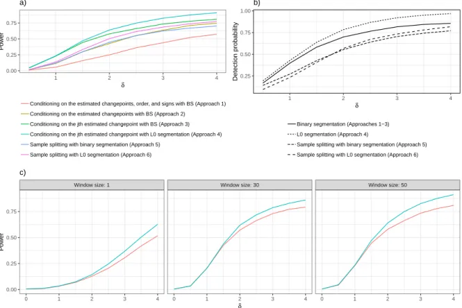
2.0, 2.5, 3.0, 3.5, 4.0}. Panel a) of Figure 3 depicts a realization with δ = 3.
We compare four different procedures for testing for a change in mean at an estimated changepoint, H0 :ν>µ= 0:
Approach 1. Conditioning on the estimated changepoints, order, and signs, {φ :
M(y0(φ)) =M(y),O(y0(φ)) =O(y),∆(y0(φ)) = ∆(y)}, for binary segmentation;
Approach 2. Conditioning on all of the estimated changepoints, {φ : M(y0(φ)) =
M(y)}, for binary segmentation;
Approach 3. Conditioning on the jth estimated changepoint, {φ: ˆτj ∈ M(y0(φ))},
for binary segmentation;
Approach 4. Conditioning on the jth estimated changepoint, {φ: ˆτj ∈ M(y0(φ))},
for `0 segmentation.
As our aim is to compare the power of Approaches 1–4, we assume the true number of changepoints (K = 50) is known— so that both binary segmentation and`0 segmentation
estimate the same (or very similar) number of changepoints1. We also assume that the underlying noise variance (σ2 = 1) is known. In what follows, all results reported are
averaged over 100 replicate data sets. Unless stated otherwise, we take the window size for testing (14) to be h = 50. In Approaches 1–3, we approximate the set S with ˜S as described in Proposition 4; we take|a−r|=|ar0+1|= max(10σ||ν||2,|ν>y|).
In practice, model selection techniques can be used to estimate K (Yao,1988;
Lebar-bier,2005;Arlot et al.,2012). Similarly, one can estimate the noise varianceσ2 based on
the data y (Birg´e and Massart, 2001; Lebarbier, 2005). Of course, the p-values in (11) and (17) do not account for these data-driven estimates.
In Section Eof the Supplementary Materials, we present timing results for estimating changepoints as well as computing p-values using Approaches 1–4. Our algorithms are very efficient: for series of length T = 1000, estimating changepoints requires less than 0.02 seconds; calculatingp-values requires less than 15 seconds in the case of Approach 4, and less than 150 seconds in the case of Approaches 1–3.
6.2 Type I error control under a global null
We take δ = 0, so that µ1 = . . . =µ2000, and examine the p-values obtained from each
of the four procedures for testing H0 :ν>µ= 0 in Section6.1. Panel b) of Figure 3
dis-plays quantile-quantile plots of the observedp-value quantiles versus theoretical Unif[0,1] quantiles. The plots indicate Type I error control.
6.3 Increases in power due to smaller conditioning sets
Next, we illustrate that power increases as the size of the conditioning event decreases, by considering Approaches 1–3 from Section6.1. Each approach uses binary segmentation; the only difference is in the size of the conditioning sets.
On a given dataset, we define the empirical power as the ratio between the number of true changepoints for which the nearest estimated changepoint has a p-value less than α and is within ±m timepoints, and the number of true changepoints,
\
Power :=
PK
i=11(|τi−τˆj(i)|≤mandpj(i)≤α)
K . (30)
Here, j(i) = argmin1≤l≤K|τi−τˆl|. Panel c) of Figure 3 shows the empirical power for
each of the four approaches with α = 0.05 and m = 2. As the size of the conditioning set decreases, the power increases substantially: the power increases by up to 15% when we condition on {φ :M(y0(φ)) = M(y)} instead of {φ : M(y0(φ)) =M(y),O(y0(φ)) =
O(y),∆(y0(φ)) = ∆(y)}, and it increases by another 20% when we condition on {φ : ˆτ j ∈
M(y0(φ))} instead of{φ :M(y0(φ)) = M(y)}.
6.4 Power and detection probability
We now compare the performances of Approaches 1–4, defined in Section 6.1, as well as two additional approaches that are based on sample splitting (Cox, 1975):
Approach 6. Apply`0segmentation to the odd timepoints to estimate changepoints.
Then apply a standard z-test of H0 :ν>µ= 0 on the even timepoints.
Because sample splitting involves estimating the changepoints on half of the data and testing for a change in mean using the other half of the data, thep-value resulting from a standard z-test for a change in mean is valid, but is conditional on the set of timepoints used to estimate the changepoints (Fithian et al., 2014).
In addition to calculating the empirical power (30) for each approach, we also consider each approach’s ability to detect the true changepoints. This is defined as the fraction of true changepoints for which there is an estimated changepoint within±m timepoints,
\
Detection probability :=
PK
i=11(min1≤l≤K|τi−τˆl|≤m)
K . (31)
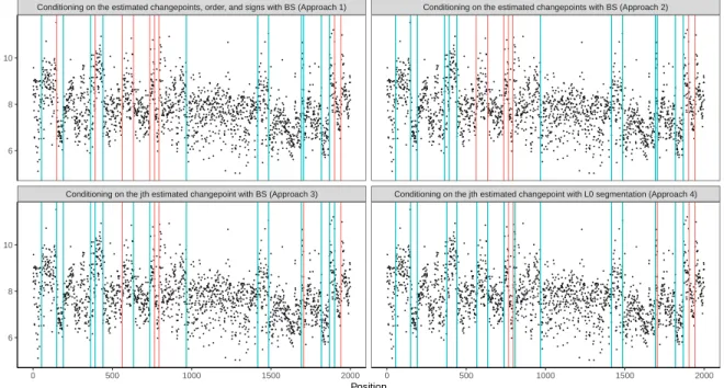
Figure 4 displays the power and detection probability for Approaches 1–6, where α= 0.05 andm= 2. In panel a), we see that Approach 4 (which estimates changepoints via `0 segmentation, and then conditions on only thejth estimated changepoint) yields
the highest power, especially for larger values of δ. In panel b), we observe that `0
segmentation vastly outperforms binary segmentation in terms of its ability to detect true changepoints.
Additionally, Figure 4 illustrates the benefit of the inferential framework developed in this paper over naive sample-splitting approaches. Sample splitting is limited in its ability to detect changepoints, since only half of the data is used to estimate changepoints.
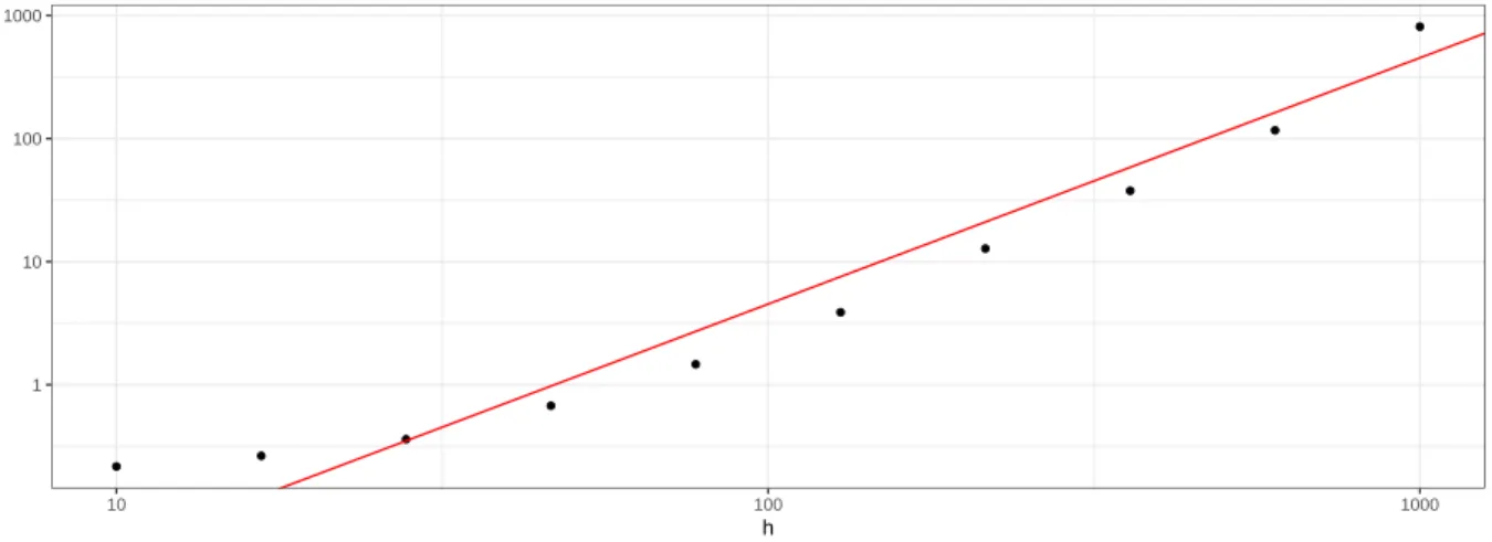
6.5 Assessment of different window sizes for testing (14)
The results in Figure4 suggest that conditioning on just ˆτj ∈ M(y0(φ)) as in (17) yields
the greatest power to detect a difference in means around ˆτj. However, this requires
pre-specifying the window size in (14). We now address this possible weakness. For window sizes h ∈ {1,30,50}, we assess the performance of Approaches 3 and 4 from Section6.1
in panel c) of Figure 4. We observe that, provided h is large enough, the window size has little effect on the power.
7 Real data example
We now consider guanine-cytosine (G-C) content on a 2Mb window of human chromo-some one, binned so that T = 2000. Data was originally accessed from the National Center for Biotechnology Information, and is available via theR packagechangepoint.
We estimate changepoints using 20-step binary segmentation, and`0segmentation
us-ing the penaltyλ = 2ˆσ2logT, which yields 20 estimated changepoints. Figure5displays
Approaches 1–4 from Section6.1 resulted in ap-value below 0.05. We see that the num-ber of discoveries (estimated changepoints whose p-value is less than 0.05) increases as the size of the conditioning set decreases. In Approach 1 we make 11 discoveries, in Approach 2 we make 13, and in Approaches 3 and 4 we make 15 discoveries.
8 Discussion
In this paper, we show that testing for a change in mean around an estimated changepoint simply requires characterizing the set S, defined in either (13) or (18). We introduce the necessary computational tools to do this for three popular changepoint detection algorithms. Importantly, since our approach does not rely on the polyhedral lemma of
Lee et al.(2016), the conditioning sets that we use are much smaller than those in earlier
work and lead to higher-powered tests. We now discuss a few extensions of our work.
8.1 Smaller conditioning sets for (10)
Similarly to Liu et al. (2018), we note that no special properties of the conditioning set were used in the proof of Theorem 1. For instance, instead of conditioning on the full set of changepoints as is done in Section 3.1, we could have instead conditioned on the jth estimated changepoint and its immediate neighbors. This would yield a p-value of the form p = Pr |φ| ≥ |ν>y| | {τˆj−1,τˆj,τˆj+1} ⊂ M(y0(φ))
, and requires only a minor modification to the algorithms in Sections 4and 5 and in the Supplemental Materials.
For some conditioning sets and changepoint detection algorithms, it might be difficult to characterizeS. In this case, it is still possible to approximateS by testing whether or not φ∈ S for a fine grid ofφ values; this approach is also suggested byLiu et al.(2018).
8.2 Confidence intervals for the change in mean
To construct confidence intervals for the change in mean, we first defineH0(c) :νTµ=c.
We note that since C(φ) = c | PrH0(c) |φ| ≥ |ν>y| |φ ∈ S
≥α satisfies Pr(ν>µ ∈
C(φ)|φ ∈ S) ≥ 1 − α, the set C(φ) is a 100(1− α)% confidence interval for ν>µ.
Importantly, we can efficiently calculate C(φ) since the set S is unchanged as we varyc; only the mean of the null distribution for ν>Y changes.
8.3 P-values for spikes obtained from calcium imaging data
The ideas in this paper apply beyond the change-in-mean model (1). In particular, the ideas in Section 3 only require conditioning on the sufficient statistics of ν>Y.
observed fluorescence trace for a neuron, yt, is a noisy version of the underlying calcium
concentration,ct, which decays exponentially with a rateγ <1, except when there is an
instantaneous increase in the calcium because the neuron has fired, st>0:
Yt =ct+t, tiid∼N(0, σ2), ct =γct−1 +st.
In this model, scientific interest lies in determining the precise timepoints of the spikes.
Jewell and Witten (2018) andJewell et al. (2019) estimate the spikes by solving
minimize
c1,...,cT
(
1 2
T
X
t=1
(yt−ct)2+λ T
X
t=2
1(ct−γct−1≥0) )
, (32)
which is closely related to the `0 segmentation problem (4) in Section 2.1.2. The
frame-work from Section 3can be used to test the null hypothesis that there is no increase in the calcium concentration around a spike, H0 : ν>c= 0, for a suitably chosen contrast
ν. Furthermore, the algorithms developed in Section 5 can be modified to efficiently characterize the selective distribution; we leave the details to future work.
Acknowledgments
We thank Zaid Harchaoui and Ali Shojaie for helpful conversations, and Jacob Bien for thoughtful suggestions based on an early version of this paper.
References
Anastasiou, A. and Fryzlewicz, P. (2019). Detecting multiple generalized change-points by isolating single ones. arXiv preprint arXiv:1901.10852.
Arlot, S., Celisse, A., and Harchaoui, Z. (2012). A kernel multiple change-point algorithm via model selection. arXiv preprint arXiv:1202.3878.
Auger, I. E. and Lawrence, C. E. (1989). Algorithms for the optimal identification of segment neighborhoods. Bulletin of Mathematical Biology, 51(1):39–54.
Badagi´an, A. L., Kaiser, R., and Pe˜na, D. (2015). Time series segmentation procedures to detect, locate and estimate change-points. In Empirical Economic and Financial Research, pages 45–59. Springer.
Bai, J. and Perron, P. (2003). Computation and analysis of multiple structural change models. Journal of Applied Econometrics, 18(1):1–22.
Barber, R. F., Cand`es, E. J., et al. (2015). Controlling the false discovery rate via knockoffs. The Annals of Statistics, 43(5):2055–2085.
Benjamini, Y. and Hochberg, Y. (1995). Controlling the false discovery rate: a practical and powerful approach to multiple testing. Journal of the Royal Statistical Society: Series B (Methodological), 57(1):289–300.
Benjamini, Y., Yekutieli, D., et al. (2001). The control of the false discovery rate in multiple testing under dependency. The Annals of Statistics, 29(4):1165–1188.
Birg´e, L. and Massart, P. (2001). A generalized Cp criterion for gaussian model selection.
Candes, E., Fan, Y., Janson, L., and Lv, J. (2018). Panning for gold:‘model-X’ knockoffs for high dimensional controlled variable selection. Journal of the Royal Statistical Society: Series B (Statistical Methodology), 80(3):551–577.
Cox, D. R. (1975). A note on data-splitting for the evaluation of significance levels.
Biometrika, 62(2):441–444.
Dombeck, D. A., Khabbaz, A. N., Collman, F., Adelman, T. L., and Tank, D. W. (2007). Imaging large-scale neural activity with cellular resolution in awake, mobile mice. Neuron, 56(1):43–57.
Fearnhead, P., Maidstone, R., and Letchford, A. (2019). Detecting changes in slope with anL0 penalty. Journal of Computational and Graphical Statistics, 28(2):265–275.
Fithian, W., Sun, D., and Taylor, J. (2014). Optimal inference after model selection.
arXiv preprint arXiv:1410.2597.
Fithian, W., Taylor, J., Tibshirani, R., and Tibshirani, R. (2015). Selective sequential model selection. arXiv preprint arXiv:1512.02565.
Frick, K., Munk, A., and Sieling, H. (2014). Multiscale change point inference. Journal of the Royal Statistical Society: Series B (Statistical Methodology), 76(3):495–580.
Friedrich, J., Zhou, P., and Paninski, L. (2017). Fast online deconvolution of calcium imaging data. PLoS computational biology, 13(3):e1005423.
Futschik, A., Hotz, T., Munk, A., and Sieling, H. (2014). Multiscale DNA partitioning: statistical evidence for segments. Bioinformatics, 30(16):2255–2262.
Harchaoui, Z. and L´evy-Leduc, C. (2007). Catching change-points with lasso. In NIPS, volume 617, page 624.
Haynes, K., Fearnhead, P., and Eckley, I. A. (2017). A computationally efficient nonpara-metric approach for changepoint detection.Statistics and Computing, 27(5):1293–1305.
Hocking, T. D., Rigaill, G., Fearnhead, P., and Bourque, G. (2018). Generalized func-tional pruning optimal partitioning (gfpop) for constrained changepoint detection in genomic data. arXiv preprint arXiv:1810.00117.
Hotz, T., Sch¨utte, O. M., Sieling, H., Polupanow, T., Diederichsen, U., Steinem, C., and Munk, A. (2013). Idealizing ion channel recordings by a jump segmentation multiresolution filter. IEEE transactions on NanoBioscience, 12(4):376–386.
Hyun, S., G’Sell, M., and Tibshirani, R. J. (2016). Exact post-selection inference for changepoint detection and other generalized lasso problems. arXiv preprint arXiv:1606.03552.
Hyun, S., Lin, K., G’Sell, M., and Tibshirani, R. J. (2018). Post-selection inference for changepoint detection algorithms with application to copy number variation data.
arXiv preprint arXiv:1812.03644.
Jackson, B., Scargle, J. D., Barnes, D., Arabhi, S., Alt, A., Gioumousis, P., Gwin, E., Sangtrakulcharoen, P., Tan, L., and Tsai, T. T. (2005). An algorithm for optimal partitioning of data on an interval. IEEE Signal Processing Letters, 12(2):105–108.
Jewell, S. and Witten, D. (2018). Exact spike train inference via `0 optimization. The
Annals of Applied Statistics, 12(4):2457.
Jewell, S. W., Hocking, T. D., Fearnhead, P., and Witten, D. M. (2019). Fast nonconvex deconvolution of calcium imaging data. Biostatistics. kxy083.
Killick, R., Fearnhead, P., and Eckley, I. A. (2012). Optimal detection of changepoints with a linear computational cost. Journal of the American Statistical Association, 107(500):1590–1598.
Lebarbier, ´E. (2005). Detecting multiple change-points in the mean of gaussian process by model selection. Signal Processing, 85(4):717–736.
Li, H., Munk, A., Sieling, H., et al. (2016). FDR-control in multiscale change-point segmentation. Electronic Journal of Statistics, 10(1):918–959.
Liu, K., Markovic, J., and Tibshirani, R. (2018). More powerful post-selection inference, with application to the lasso. arXiv preprint arXiv:1801.09037.
Ma, T. F. and Yau, C. Y. (2016). A pairwise likelihood-based approach for changepoint detection in multivariate time series models. Biometrika, 103(2):409–421.
Maidstone, R., Hocking, T., Rigaill, G., and Fearnhead, P. (2017). On optimal multiple changepoint algorithms for large data. Statistics and Computing, 27(2):519–533.
Muggeo, V. M. and Adelfio, G. (2010). Efficient change point detection for genomic sequences of continuous measurements. Bioinformatics, 27(2):161–166.
Niu, Y. S. and Zhang, H. (2012). The screening and ranking algorithm to detect DNA copy number variations. The Annals of Applied Statistics, 6(3):1306.
Olshen, A. B., Venkatraman, E., Lucito, R., and Wigler, M. (2004). Circular binary segmentation for the analysis of array-based dna copy number data. Biostatistics, 5(4):557–572.
Rigaill, G. (2015). A pruned dynamic programming algorithm to recover the best segmen-tations with 1 to Kmax change-points. Journal de la Soci´et´e Fran¸caise de Statistique,
156(4):180–205.
Rudin, L. I., Osher, S., and Fatemi, E. (1992). Nonlinear total variation based noise removal algorithms. Physica D: Nonlinear Phenomena, 60(1-4):259–268.
Schr¨oder, A. L. and Fryzlewicz, P. (2013). Adaptive trend estimation in financial time series via multiscale change-point-induced basis recovery. Statistics and Its Interface, 4(6):449–461.
Tian, X., Taylor, J., et al. (2018). Selective inference with a randomized response. The Annals of Statistics, 46(2):679–710.
Tibshirani, R., Saunders, M., Rosset, S., Zhu, J., and Knight, K. (2005). Sparsity and smoothness via the fused lasso. Journal of the Royal Statistical Society: Series B (Statistical Methodology), 67(1):91–108.
Vogelstein, J. T., Packer, A. M., Machado, T. A., Sippy, T., Babadi, B., Yuste, R., and Paninski, L. (2010). Fast nonnegative deconvolution for spike train inference from population calcium imaging. Journal of Neurophysiology, 104(6):3691–3704.
Vostrikova, L. (1981). Detection of the disorder in multidimensional random-processes.
Doklady Akademii Nauk SSSR, 259(2):270–274.
Xiao, F., Luo, X., Hao, N., Niu, Y. S., Xiao, X., Cai, G., Amos, C. I., and Zhang, H. (2019). An accurate and powerful method for copy number variation detection.
Bioinformatics.
Yao, Y.-C. (1988). Estimating the number of change-points via Schwarz’criterion. Statis-tics & Probability Letters, 6(3):181–189.
−10 −5 0 5
0 50 100 150 200
a)
−10 −5 0 5
0 50 100 150 200
b)
Figure 1: The power of a test of (9) critically depends on the size of the conditioning set. Observations (displayed in grey) were simulated from (1) withσ = 1 andµ1, . . . , µT
displayed in dark blue. Our proposed test of (9) was conducted for each of the change-points estimated via 19-step binary segmentation. Estimated changechange-points for which the p-value is less than 0.05 are displayed in blue, and the remaining estimated changepoints are displayed in red. In panel (a), we conducted our proposed test by conditioning on
M(Y) = M(y),O(Y) = O(y),∆(Y) = ∆(y), and Π⊥
νY = Π⊥νy (this is essentially the
proposal of Hyun et al. (2018)). In panel (b), we conditioned on the much smaller set
M(Y) =M(y) and Π⊥
Figure 2: a) A simulated dataset with φ = ν>y = −1 is displayed in grey, and the true underlying mean is shown in blue. b) The perturbed dataset y0(φ) is shown, with
φ = ν>y = 0. The perturbed dataset does not have a change in mean at the 100th
timepoint, and so 1-step binary segmentation does not detect a changepoint at that position. c) The perturbed dataset y0(φ) is shown, with φ = ν>y = −2. There is
now a very pronounced change in mean at the 100th timepoint, and so 1-step binary segmentation does detect a changepoint at that position. d) Values of φ for which
M(y0(φ)) =M(y) are shown in blue, and those for which M(y0(φ))6=M(y) are shown
−2 0 2 4 6
0 500 1000 1500 2000
a)
Approach 1 Approach 2 Approach 3 Approach 4
0.00 0.25 0.50 0.75 1.00 0.00 0.25 0.50 0.75 1.00 0.00 0.25 0.50 0.75 1.00 0.00 0.25 0.50 0.75 1.00
0.00 0.25 0.50 0.75 1.00
Theoretical Unif[0, 1] quantiles
Obser v ed p −v alue quantiles b) ● ● ● ●●● ● ● ● ● ● ● ● ● ● ● ● ● ● ● ● ● ● ● ● ● ● 0.0 0.2 0.4 0.6 0.8
0 1 2 3 4
δ P o w er ● ● ●
Conditioning on the estimated changepoints, order, and signs with BS (Approach 1) Conditioning on the estimated changepoints with BS (Approach 2) Conditioning on the jth estimated changepoint with BS (Approach 3)
c)
Figure 3: a) The grey points represent a realization from the mean model (1), with true change in mean due to a changepoint δ = 3. The mean µ1, . . . , µT is shown as a
blue line, and the changepoints are shown as grey vertical lines. b) The panels display quantile-quantile plots comparing sample p-value quantiles under (1) with µ1 = . . . =
µ2000 versus theoretical quantiles of the Unif(0,1) distribution, for the four approaches
listed in Section 6.1. c) Empirical power, averaged over 100 replicates, is displayed for Approaches 1–3 defined in Section 6.1, each of which results from testing H0 :ν>µ= 0
0.00 0.25 0.50 0.75
1 2 3 4
δ
P
o
w
er
Conditioning on the estimated changepoints, order, and signs with BS (Approach 1)
Conditioning on the estimated changepoints with BS (Approach 2)
Conditioning on the jth estimated changepoint with BS (Approach 3) Conditioning on the jth estimated changepoint with L0 segmentation (Approach 4)
Sample splitting with binary segmentation (Approach 5)
Sample splitting with L0 segmentation (Approach 6)
a)
0.25 0.50 0.75 1.00
1 2 3 4
δ
Detection probability
Binary segmentation (Approaches 1−3) L0 segmentation (Approach 4)
Sample splitting with binary segmentation (Approach 5)
Sample splitting with L0 segmentation (Approach 6)
b)
Window size: 1 Window size: 30 Window size: 50
0 1 2 3 4 0 1 2 3 4 0 1 2 3 4
0.00 0.25 0.50 0.75
δ
P
o
w
er
Conditioning on the jth estimated changepoint with BS (Approach 3) Conditioning on the jth estimated changepoint with L0 segmentation (Approach 4)
c)
Figure 4: Empirical power and detection probability for different changepoint estima-tion and inference procedures. a) Power for Approaches 1–4, which are described in Section6.1, as well as Approaches 5–6, which are described in Section 6.4. b) Detection probability for binary segmentation and`0 segmentation using all of the data, as well as
Conditioning on the jth estimated changepoint with BS (Approach 3) Conditioning on the jth estimated changepoint with L0 segmentation (Approach 4) Conditioning on the estimated changepoints, order, and signs with BS (Approach 1) Conditioning on the estimated changepoints with BS (Approach 2)
0 500 1000 1500 2000 0 500 1000 1500 2000
6 8 10
6 8 10
Position
G−C content
Figure 5: The number of discoveries depends on the size of the conditioning set. Scaled G-C content on a 2Mb window of human chromosome one. The G-C content is binned leading to T = 2000 (displayed in black). Changepoints are estimated via 20-step binary segmentation, and `0 segmentation with tuning parameter λ = 2ˆσ2log(2000) ≈ 5.5.
Supplementary Materials:
Testing for a Change in Mean After
Changepoint Detection
Sean Jewell
∗Department of Statistics, University of Washington
Paul Fearnhead
Department of Mathematics and Statistics, Lancaster University
Daniela Witten
Departments of Statistics and Biostatistics, University of Washington
A Proof of Theorem 1
To characterize (10), we note that Y decomposes as
Y = (I−Π⊥ν)Y + Π⊥νY, (A1)
where Π⊥
ν =I− νν
>
||ν||2
2. Then (10) becomes
p= PrH0 |ν
>Y| ≥ |ν>y| | M(Y) = M(y),Π⊥
νY = Π⊥νy
(A2) = PrH0 |ν
>Y| ≥ |ν>y| | M((I−Π⊥
ν)Y + Π⊥νy) = M(y),Π⊥νY = Π⊥νy
(A3) = PrH0 |ν>Y| ≥ |ν>y| | M((I−Π⊥ν)Y + Π⊥νy) = M(y)
. (A4)
∗Sean Jewell received funding from the Natural Sciences and Engineering Research Council of
Canada. This work was partially supported by Engineering and Physical Sciences Research Council Grant EP/N031938/1 to Paul Fearnhead, and NSF CAREER DMS-1252624, NIH grants DP5OD009145, R01DA047869, and R01EB026908, and a Simons Investigator Award in Mathematical Modeling of Living Systems to Daniela Witten.
1
Here, (A2) is our definition of ap-value (10), and (A3) follows from (A1) and the fact that Π⊥
νY = Π⊥νy. Finally, (A4) follows from the fact thatY is Gaussian (see (1)) and so ν>Y
and Π⊥
νY are independent.
Moreover, we note that (1) implies that ν>Y ∼ N(ν>µ,kνk2σ2), and that under the
null hypothesis (9), ν>Y ∼ N(0,kνk2σ2). We now define φ = ν>Y; thus under the null
hypothesis, φ∼N(0,kνk2σ2). Recall that
y0(φ) = y− νν>y ||ν||2 2
+ νφ
||ν||2 2
. (A5)
Therefore,
p= Pr |φ| ≥ |ν>y| | M(y0(φ)) =M(y). (A6)
B Details related to Section 4
B.1 Proof of Proposition 2
To prove the first statement in Proposition 2, we note from Proposition 1 that the set of data that yields changepoints m, orders o, and signs d is of the form {y : Γy ≤ 0}. Therefore, the set of φ that yields M(y0(φ)) =m,O(y0(φ)) =o, and ∆(y0(φ)) =d is of the
form {φ: Γy0(φ) ≤0}. Since Γy0(φ)≤0 represents k(2T −k−3) linear inequalities in φ,
the set {φ:Γy0(φ)≤0} is an interval.
The second statement in Proposition 2 follows from the fact that
S = [
o∈O,d∈D
{φ:M(y0(φ)) = M(y),O(y0(φ)) =o,∆(y0(φ)) =d} (B7)
= [
(o0,d0)∈I
{φ:M(y0(φ)) =M(y),O(y0(φ)) =o0,∆(y0(φ)) =d0} (B8)
=
N0
[
i=−N
(ai, ai+1) (B9)
where O is the set of cardinality k! containing all possible orders of the k changepoints, and D:={−1,+1}k is the set of possible signs. Recall that N0+N+ 1 =|I| forI defined
in (21).
A key insight of (B7)-(B9) is that (B7) is the union over 2kk! intervals. By contrast,
(B9) is a union is over N0 +N + 1 = |I| intervals which in practice is much smaller than 2kk!.
B.2 Proof of Proposition 4
To prove Proposition 4, recall that S = SNi=−N0 (ai, ai+1), as described in Section 4, where
a−N =−∞andaN0 =∞. Also recall that ˜S = (−∞, a−r)∪nSr 0
i=−r(ai, ai+1)
o
∪(ar0+1,∞),
for somea−r ≤ −|ν>y|andar0+1 ≥ |ν>y|. Since{|φ| ≥ |ν>y|} ∩ {φ ∈S \ S}˜ ={φ ∈S \ S}˜ ,
we have
Pr(|φ| ≥ |ν>y| |φ∈S˜) = Pr({|φ| ≥ |ν
>y|} ∩ {φ∈S}˜ )
Pr(φ∈S˜)
= Pr({|φ| ≥ |ν>y|} ∩ {φ∈ S}) + Pr({|φ| ≥ |ν>y|} ∩ {φ∈S \ S}˜ ) Pr(φ∈ S) + Pr(φ ∈S \ S˜ )
= Pr({|φ| ≥ |ν
>y|} ∩ {φ∈ S}) + Pr(φ ∈S \ S˜ )
Pr(φ∈ S) + Pr(φ ∈S \ S˜ )
≥Pr(|φ| ≥ |ν>y| |φ ∈ S).
B.3 Characterization of (18)
In this section, we show that we can characterize the set S ≡ {φ : ˆτj ∈ M(y0(φ))} for
changepoints estimated via binary segmentation. Our approach is very similar to that of Section 4. In the following two propositions, Propositions B1 and B2, we modify Proposi-tions 2 and 3 for the case of S defined in (18).
Proposition B1 The set {φ :M(y0(φ)) =m,O(y0(φ)) =o,∆(y0(φ)) =d} is an interval.
Furthermore, the set S defined in (18) can be written as the union of intervals,
S ={φ : ˆτj ∈ M(y0(φ))}= N0
[
i=−N
(ai, ai+1), (B10)
where N0+N + 1 is the number of elements in the set
I :={(o, d) :∃α∈R such that o=O(y0(α)), d= ∆(y0(α)),τˆj ∈ M(y0(α))}. (B11)
I is the set of possible orders and signs of the changepoints that can be obtained via a perturbation of y that yields a changepoint at τˆj.
Proposition B2 SNi=0−N(ai, ai+1) defined in (B10) can be efficiently computed.
We outline the proof for PropositionB2here. We first runk-step binary segmentation on the data y in order to obtain estimated changepointsM(y), orders O(y), and signs ∆(y). We then apply the first statement in Proposition B1 to obtain an interval [a0, a1] ⊂ S.
Next, for some small positive value of η, we apply the first statement of Proposition B1
with m=M(y0(a
1+η)), o=O(y0(a1+η)), and d= ∆(y0(a1+η)) to identify the interval
[a1, a2]. We then check whether ˆτj ∈ M(y0(a1 +η)); if so, then [a1, a2] ⊂ S, and if not,
then [a1, a2]6⊂ S. We continue in this vein, much as we did in Section 4, to obtain the full
set S.
In fact, when characterizing the set S = {φ : ˆτj ∈ M(y0(φ))}, this procedure can be
sped up. We first define the interval in φ such that j-step binary segmentation yields the estimated changepoints m, orderso, and signs d
{φ:Mj(y0(φ)) =m,Oj(y0(φ)) =o,∆j(y0(φ)) =d}, (B12)
where the subscripts indicate that we have used j-step binary segmentation as opposed to k-step binary segmentation.
Now, recall that ˆτj is thejth estimated changepoint resulting from binary segmentation
on the data y. Suppose that j < k. We first run j-step binary segmentation on y in order to obtain estimated changepoints Mj(y), orders Oj(y), and signs ∆j(y). Then we can
identify an interval [a0, a1] ⊂ S by applying (B12) with m = Mj(y), o = Oj(y), and
d = ∆j(y). This leads to substantial computational speed-ups if j k. Next, suppose
that ˆτj is thelth estimated changepoint resulting fromk-step binary segmentation applied
to y0(a
1+η), for l < k. Once again, we can identify an interval [a1, a2] ⊂ S by applying
(B12) with m=Ml(y0(a1+η)),o =Ol(y0(a1+η)), and d= ∆l(y0(a1+η)). By contrast, if
ˆ
τj ∈ M/ k(y0(a1+η)) or if ˆτj is the kth estimated changepoint on the data y0(a1+η), then
we must identify intervals using the first statement of Proposition B1.
C Details related to Section 5
C.1 Proof of Theorem 2
To compute Cost(y0
1:s(φ);u) fors ∈ {τˆj−1+ 1, . . . ,τˆj+1}, we will introduce a set of functions
Cs; each function in the set will correspond to a possible configuration for the changepoints
preceding thesth timepoint. Then, Cost(y0
1:s(φ);u) = minf∈Csf(u, φ). Importantly, we will
construct the set Cs in such a way that its size grows linearly, rather than exponentially,
in the size of the set of values that s can take.