XXX-X-XXXX-XXXX-X/XX/$XX.00 ©20XX IEEE
Deep Rule-Based Aerial Scene Classifier using
High-Level Ensemble Feature Descriptor
Xiaowei Gu 1,2 1
School of Computing and
Communications, 2
Lancaster Intelligent, Robotic and Autonomous systems (LIRA)
Research Centre, Lancaster University
Lancaster, UK [email protected]
Plamen P. Angelov 1,2 1
School of Computing and
Communications, 2
Lancaster Intelligent, Robotic and Autonomous systems (LIRA)
Research Centre, Lancaster University
Lancaster, UK [email protected]
Abstract—In this paper, a new deep rule-based approach
using high-level ensemble feature descriptor is proposed for aerial scene classification. By creating an ensemble of three pre-trained deep convolutional neural networks as the feature descriptor, the proposed approach is able to extract more discriminative representations from the local regions of aerial images. With a set of massively parallel IF…THEN rules built upon the prototypes identified through a self-organizing, nonparametric, transparent and highly human-interpretable learning process, the proposed approach is able to produce the state-of-the-art classification results on the unlabeled images outperforming the alternatives. Numerical examples on benchmark datasets demonstrate the strong performance of the proposed approach.
Keywords— deep rule-based, deep convolutional neural network, ensemble feature descriptor, aerial scene classification
I. INTRODUCTION
Aerial images are an important source of information for people to understand the Earth [1]. Aerial scene classification is currently a hot research topic because it is instrumental for many real-world applications [2]. Meanwhile, this task is very challenging due to the highly complex semantic contents and spatial patterns of such images.
There have been many approaches proposed for classifying the aerial images. In general, they can be divided into three
main categories [3]: 1) low-level methods; 2) middle-level
methods; and 3) high-level methods.
Low-level methods attempt to distinguish aerial scenes based on the low-level visual features extracted from the images [4]–[6]. Middle-level methods, in general, encode the low-level visual features extracted from the local regions of the aerial images into holistic middle-level representations for scene classification [7], [8]. High-level methods are, mostly, based on deep convolutional neural networks (DCNNs) [2], [9], [10]. In comparison to the former two categories, high-level methods can perform classification with the highest accuracy and are the state-of-the-art in the remote sensing domain. Nonetheless, practically all of the existing high-level methods lack transparency in the approximate reasoning process, and the reasons for making a particular decision are often not interpretable for humans [11]. These demerits largely
influence the applicability of the high-level approaches in real-world scenarios.
As a recently introduced generic approach for image classification, deep rule-based (DRB) classifier [12], [13] is a powerful alterative to the DCNN models. The DRB approach expands the traditional fuzzy rule-based (FRB) systems with a massively parallel multi-layer structure that DCNNs benefit from [13]. Thanks to the prototype-based nature, the system structure of the DRB approach is fully transparent, and the learning and decision-making processes are autonomous, nonparametric and highly interpretable for humans [11].
The DRB classifier may employ different types of descriptors for visual feature extraction, which can be low-level [14], [15], middle-low-level [8] or high-low-level [16]–[18]. In reality, however, using one type of feature is often not enough for classifying different scene categories that share similar appearances. Different feature descriptors have different merits and demerits, and they have different descriptive abilities. Therefore, fusing multiple features into more descriptive representations usually results in a stronger classification performance [1], [19], [20].
Following this principle, in this paper, a deep rule-based (DRB) approach using multiple features is proposed for aerial scene classification. The proposed approach uses an ensemble of different high-level feature descriptors for extracting highly distinctive semantic representations from sub-regions of aerial images locally. The DRB system identifies a number of prototypes during the training process, and self-organizes a set of massively parallel prototype-based IF…THEN rules for classification in an autonomous, nonparametric manner [11]– [13]. Numerical examples demonstrate that the proposed DRB approach is able to produce the state-of-the-art classification results outperforming the alternatives by incorporating the high-level ensemble feature descriptor.
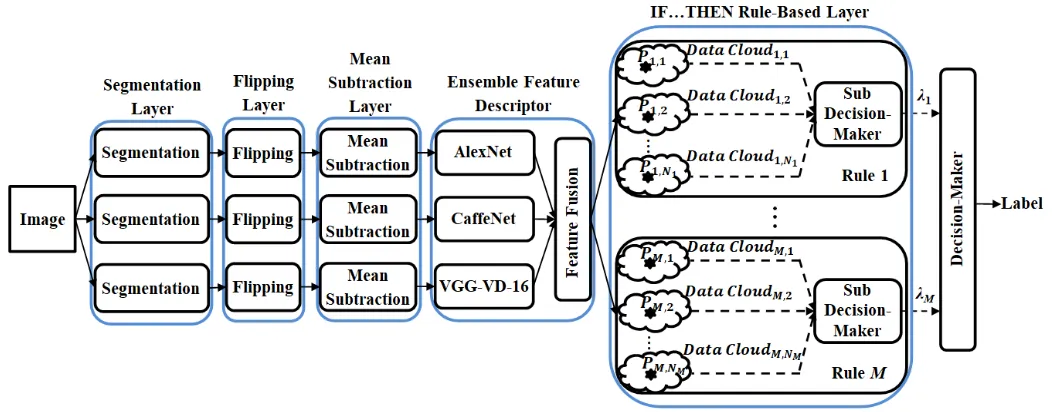
II. THE EMPLOYED HIGH-LEVEL FEATURE DESCRIPTORS
Fig. 1. The general architecture of the proposed DRB approach Fig. 1.
Fig. 2. A. AlexNet
AlexNet [18] was the winning DCNN model of the ImageNet Large Scale Visual Recognition Challenge (ILSVRC) in 2012. It largely popularized the applications of DCNNs and has become a baseline model of DCNNs. AlexNet was trained on ImageNet dataset, which contains 1.3 million images. It has eight layers with weights. The first five are convolutional layers, the first and second of which are followed by the normalization layers. The two normalization layers and the fifth convolutional layer are also followed by one max-pooling layer, respectively. The remaining three layers with weights are connected [18]. The last fully-connected layer is linked to a softmax layer which produces the output of the network. To reduce overfitting, AlexNet involves data augmentation by cropping smaller-size segments and horizontally flipping these segments from original images. This operation artificially creates more training images. The
size of input images required by AlexNet is227 227 pixels.
In this paper, we use the 1 4096 dimensional activations
from the first fully connected layer as the feature vectors of the input images.
B. CaffeNet
CaffeNet [16] has a similar architecture to AlexNet and is also trained on the image set of ILSVRC 2012. Nonetheless, there are two differences between CaffeNet and AlexNet [3]:
1) the order of max-pooling and normalization layers are
exchanged; 2) data augmentation is not used. The size of input
images required by CaffeNet is227 227 pixels. Similarly, the
1 4096 dimensional activations from the first fully connected layer are used as the feature vector of the input images [2].
C. VGG-VD-16 Model
VGG-VD-16 was introduced in [17] and is one of the best-performing pre-trained DCNN models. This model has 16 layers with weights. The first 13 layers are convolutional and the last three are fully-connected. The second, fourth, seventh,
tenth, thirteenth convolutional layers are followed by a max-pooling layer. There is no normalization layer used in the VGG-VD-16 model. This model is also trained on the image set of ILSVRC 2012 [17]. VGG-VD-16 model requires the
input images with the size of 224 224 pixels. We also extract
the 1 4096 dimensional activations from the first fully connected layer as the feature vectors of the input images [2].
It has to be stressed that, practically, one can use any types of high-level feature descriptors, i.e. GoogLeNet [21], ResNet [22], PlacesNet [23], etc., and any number of them to create an ensemble for feature extraction. The main purpose of this paper, however, is to introduce the general concept and principles of the DRB classifier using ensemble feature descriptor. Therefore, we only use the most representative three DCNNs to create the ensemble descriptor. Nonetheless, one can try different combinations as well.
III. THE PROPOSED DEEP RULE-BASED APPROACH
The general architecture of the proposed DRB approach is depicted in Fig. 1. As one can see that, the DRB classifier is composed of the following layers:
1) Segmentation layer;
2) Flipping layer;
3) Mean subtraction layer;
4) Ensemble feature descriptor layer;
5) IF…THEN rule-based layer;
6) Decision-maker.
A. Segmentation Layer
This layer crops five sub-images of the required sizes
( 224 224 or 227 227 pixels depending on the DCNN
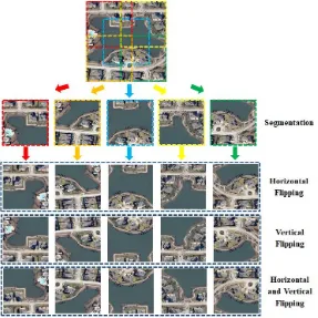
Fig. 2. Illustrative example of data augmentation
semantic information from the images and improve the generalization ability.
B. Flipping Layer
This layer flips each segment of the images horizontally, vertically, and in both direction. The flipping operation further creates three new segments from each segment [2], [18].
The segmentation and flipping layers, in total,
produce Ko20 segments from each input image,
which will be used for feature extraction. An example of the data augmentation is given in Fig. 2 for illustration.
C. Mean Subtraction Layer
This layer subtracts from each segment its mean, and centralizes the three channels of the segment around the zero mean. This pre-processing technique helps the pre-trained DCNN models to perform faster because gradients act uniformly for each channel.
D. Ensemble Feature Descriptor Layer
The ensemble feature descriptor, as described in Section II, consists of three different pre-trained
DCNN models: 1) AlexNet, 2) CaffeNet and 3)
VGG-VD-16, and a feature fusion sub-layer.
For each segment, denoted by s, each model will
produce a 1 4096 dimensional feature vector from the
activations of the first fully connected layer. The feature fusion sublayer will combine the three feature vectors into a
1 12288 dimensional semantic representation by the following equation:
,
,
T
AN s CN s VV s
AN s CN s VV s
x (1)
where AN s
, CN s
, VV s
represent the feature vectorsextracted by AlexNet, CaffeNet and VGG-VD-16 models,
respectively. In equation (1), L2-normalization is used to
guarantee that the feature vectors from the three models contribute equally in the semantic representation.
E. IF…THEN Rule-Based Layer
The IF…THEN rule base in this layer is the “core” of the
DRB classifier. Assuming the datasets has M categories, the
DRB classifier will self-organize and self-update M
massively parallel IF…THEN rules from prototypes that are identified from the segments of the images of each category (one rule per category) in a nonparametric, transparent and human-interpretable manner. Each IF…THEN rule has the
following form (m1, 2,...,M) [11]–[13]:
,1 ,2 ,
~ ~ ... ~
m
m m m N
IF OR OR OR
THEN category m
s P s P s P
(2)
where “ ~ ” denotes similarity, which can be seen as a fuzzy
degree of membership; s is a particular segment with xas its
feature vector; Pm i, denotes the ith prototype of the mth category
with pm i, as the corresponding feature vector; Nm is the
number of identified prototypes of the mth category.
Each IF…THEN rule contains a number of prototypes that are connected by a sub-decision maker using the “winner-takes-all” principle. Therefore, each IF…THEN rule is a massively parallel series of singleton fuzzy rules of AnYa type [24] connected by logical “OR” operators .
The detailed identification process of the IF…THEN rules have been given in [11], [13]. One can also download from [25] the open source software implemented in Matlab with detailed instructions provided in [11]. To make this paper self-contained, the identification process of the rule base is summarized by the following pseudo-code. It has to be noticed that because the IF…THEN rules are identified in parallel, we
present the identification process of the mth rule as an example.
The same principles can be applied to the other IF…THEN rules within the same rule base.
INPUT: streaming images of the mth category
ALGORITHM BEGINS
While a new segment, sm k, is available:
i. Extract the semantic representation, xm k, from sm k, ;
, , , m k m k m k x x
x (2)
iii. If (k1) Then
1. Initialize the global meta-parameters:
,
1;
m m m k
N
x (3)where, Nm is the number of prototypes;
m is theglobal mean of the feature vectors of the images of
the mth category.
2. Initialize the meta-parameters of the first data cloud,
, m m N
C :
, m ,
m N m k
C s (4a)
, m ,
m N m k
P s (4b)
, m ,
m N m k
p x (4c)
, m 1
m N
S (4d)
, m m N o
r r (4e)
where ,
m m N
S is the support (number of members) of
, m m N
C ; ,
m m N
r is the corresponding radius of
influential area; ro is a constant to stabilize the new
data cloud and 2 1 cos 30
o
o
r [11], [13].
3. Initialize the IF…THEN rule:
,
: ~
m
m IF m N THEN category m
R s P (5)
iv. Else
1. Update global mean:
,
1 1
m m m k
k
k k
x
(6)2. Calculate the data density at sm k, and prototypes Pm j,
(j1,...,Nm) [26], [27]:
22 1 1 1 m D z z z
(7)
where , , ,1, ,2,..., ,
m m k m m m N
z = s P P P ;
, , ,1, ,2,..., ,
m m k m m m N
z x p p p .
3. Find the nearest data cloud, Cm n, *:
, ,
1,2,...,
* arg min
m
m k m j
j N
n
x p (8)
4. If (
,
,
1,2,...,
max
m
m k m j
j N
D D
s P )
Or (
,
,
1,2,...,min m
m k m j
j N
D D
s P )
Or ( xm k, pm n, * rm n, *) Then:
- Add a new data cloud:
1
m m
N N (9a)
, m ,
m N m k
C s (9b)
, m ,
m N m k
P s (9c)
, m ,
m N m k
p x (9d)
, m 1
m N
S (9e)
, m m N o
r r (9f)
5. Else:
- Update the meta-parameters of Cm n, *:
, * , * ,
m n m n m k
C C s (10a)
, * , * , * , , * , * 1 1 1 m n
m n m n m k
m n m n
S
S S
p p x (10b)
, * , * 1
m n m n
S S (10c)
2
2
, * , *
, *
1
2
m n m n
m n r r
p (10d)
6. End If
7. Update the IF…THEN rule:
,1 ,
~ ... ~
: m m Nm
m
IF OR OR
THEN category m
s P s P
R (11)
v. End If End While
ALGORITHM ENDS
OUTPUT: the massively parallel IF…THEN rule Rm
F. Decision-Maker
During the validation process, for a particular segment, si
(i1, 2,..., 20) from an unlabelled image, I, one can obtain
M scores of confidence with the corresponding M massively
parallel IF…THEN rules (one score per rule). Each score of
confidence is formulated as follows (m1, 2,...,M ):
2, 1,2,...,
max i m j m
m i
j N e
s x p (12)
where xi is the corresponding12288 1 dimensional semantic
representation of si.
The label of I is given using the “winner takes all”
principle by combing the scores of confidence calculated with
all the segments of I:
1,2,..., 1
1
*; * arg max
o K
m i
m M o i
Label category m m
K
I s (13)
IV. NUMERICAL EXAMPLES AND DISCUSSIONS
In this section, numerical examples on well-known benchmark image sets are presented to demonstrate the performance of the proposed approach.
A. Experimental Setup
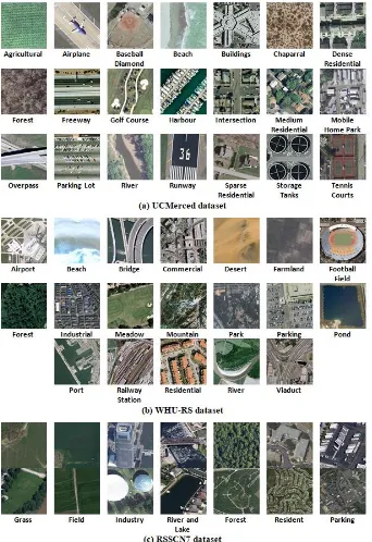
In this paper, the following three aerial image sets are used for numerical examples. The example images of the three benchmark image sets are given in Fig. 3.
Fig. 3. Illustrative example of the three benchmark problesm
UCMerced dataset consist of land-use images of 21 categories selected from aerial orthoimagery. This dataset has, in total, 2100 images of a size of
256 256 pixels. These images are uniformly labelled into the following
21 categories: i) agricultural; ii)
airplane; iii) baseball diamond; iv)
beach; v) buildings; vi) chaparral; vii)
dense residential; viii) forest; ix)
freeway; x) golf course; xi) harbour;
xii) intersection; xiii) medium
residential; xiv) mobile home park; xv)
overpass; xvi) parking lot; xvii) river;
xviii) runway; xix) sparse residential;
xx) storage tanks; and xxi) tennis
courts. UCMerced dataset has a variety of categories, some of which are highly overlapping. Therefore, it is widely used as a benchmark.
2) WHU-RS dataset [28]
WHU-RS dataset is a popular benchmark dataset collected from Google Earth (Google Inc.). It consists
of 950 images with a size of 600 600
pixels. This dataset has 19 categories,
which include i) airport; ii) beach; iii)
bridge; iv) commercial, v) desert; vi)
farmland; vii) football field; viii) forest;
ix) industrial; x) meadow; xi)
mountain; xii) park; xiii) parking lot;
xiv) pond; xv) port; xvi) railway; xvii)
residential; xviii) river; and xix)
viaduct, with 50 images in each.
WHU-RS dataset contains aerial
images with high variations in terms of illumination, scale resolution, etc., and, thus, is a difficult problem.
3) RSSCN7 dataset [9]
RSSCN7 dataset is collected from Google Earth (Google Inc.) as well. It has seven categories, and each one contains 400 images with the size of
400 400 pixels. The seven categories
include: i) grassland; ii) forest; iii)
farmland; iv) parking lot; v) resident;
vi) industry and vii) river and lake. The
images of each category are sampled as four different scales (100 images per scale) with different angles, which make this problem a challenging one.
In this paper, we rescale the images of the WHU-RS dataset into the same size of the images of the RSSCN7
dataset, namely, 400 400 pixels, to avoid the loss of
information during the segmentation operation.
For the training and validation sets separation, we follow the common practice by adopting two different sets [1], [3]. For UCMerced dataset, the ratios of the images for training per
category are set to be 50% and 80%. For WHU-RS dataset, the ratios are set to be 40% and 60%. For RSSCN7 dataset, the ratios of the training images are set to be 20% and 50% per category.
The experimental results by the proposed approach are reported in the form of:
All the results are the average after 10 times Monte Carlo experiments. A variety of the state-of-the-art approaches are selected for comparison purposes.
B. Experimental Results and Comparisons
[image:6.612.50.295.171.406.2]The experimental results on the UCMerced dataset obtained by the proposed approach as well as the selected state-of-the-art approaches are reported in Table I.
TABLE I. NUMERICAL RESULTS ON UCMERCED DATASET
Algorithm
Percentage of Training Images per Category
50% 80%
The proposed 0.9402±0.0042 0.9736±0.0086 salM3LBP-CLM [1] 0.9421±0.0075 0.9575±0.0080
salM3LBP [1] 0.8997±0.0085 0.9314±0.0100
salCLM (eSIFT) [1] 0.9293±0.0092 0.9452±0.0079 Combing Scenarios I and II [2] 0.9849
Fine-tuning GoogleNet [29] 0.9710
CaffeNet [3] 0.9398±0.0067 0.9502±0.0081 GoogLeNet [3] 0.9270±0.0060 0.9431±0.0089 VGG-VD-16 [3] 0.9414±0.0069 0.9521±0.0120 BoVW(SIFT) [3] 0.7190±0.0079 0.7412±0.0330 VLAD(SIFT) [3] 0.7323±0.0102 0.7819±0.0166 MS-CLBP+FV [30] 0.8876±0.0079 0.9300±0.0120
The experimental results obtained by the proposed
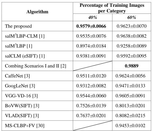
approach on the WHU-RS dataset are reported in Table II.
[image:6.612.47.296.494.708.2]Comparison with the state-of-the-art is reported in the same table as well.
TABLE II. NUMERICAL RESULTS ON WHU-RSDATASET
Algorithm
Percentage of Training Images per Category
40% 60%
The proposed 0.9579±0.0066 0.9623±0.0070 salM3LBP-CLM [1] 0.9535±0.0076 0.9638±0.0082
salM3LBP [1] 0.8974±0.0184 0.9258±0.0089
salCLM (eSIFT) [1] 0.9381±0.0091 0.9592±0.0095 Combing Scenarios I and II [2] 0.9889
CaffeNet [3] 0.9511±0.0120 0.9624±0.0056 GoogLeNet [3] 0.9312±0.0082 0.9471±0.0133 VGG-VD-16 [3] 0.9544±0.0060 0.9605±0.0091 BoVW(SIFT) [3] 0.7526±0.0139 0.8013±0.0201 VLAD(SIFT) [3] 0.7637±0.0201 0.8082±0.0215
MS-CLBP+FV [30] 0.9453±0.0102
The experimental results obtained by the proposed
approach on the RSSCN7 datasetare reported in Table III, and
are compared with the state-of-the-art in the same table.
TABLE III. NUMERICAL RESULTS ON RSSCN7DATASET
Algorithm
Percentage of Training Images per Category
20% 50%
The proposed 0.8826±0.0056 0.9175±0.0045
CaffeNet [3] 0.8557±0.0095 0.8885±0.0062 GoogLeNet [3] 0.8398±0.0087 0.8718±0.0094 VGG-VD-16 [3] 0.8255±0.0111 0.8584±0.0092 BoVW(SIFT) [3] 0.7633±0.0088 0.8134±0.0055 VLAD(SIFT) [3] 0.7727±0.0058 0.8082±0.0215
DBNFS [9] 0.7119 0.7581
In Tables I, II and III, the best results reported are highlighted.
C. Discussions
Tables I, II and III demonstrate that the proposed approach is able to produce the state-of-the-art results in all three benchmark image sets. In particular, the proposed DRB approach outperforms all other comparative approaches on the RSSCN7 dataset. Therefore, one may conclude that the proposed approach is a strong alternative to other approaches for aerial image classification.
V. CONCLUSION AND FUTURE WORK
In this paper, a new deep rule-based (DRB) approach using an ensemble of high-level feature descriptors for aerial scene classification is proposed. With the discriminative semantic representations from the sub-regions of the aerial images extracted by the ensemble feature descriptor, the DRB approach is able to produce highly accurate classification results after a nonparametric, self-organizing and human-interpretable learning process outperforming the alternatives. Numerical examples on benchmark datasets verify the proposed concept and principles.
As future work, we will investigate the performance of the DRB approach with different combinations of the high-level feature descriptors as well as different feature fusion strategies.
REFERENCES
[1] X. Bian, C. Chen, L. Tian, and Q. Du, “Fusing local and global features for high-resolution scene classification,” IEEE J. Sel. Top. Appl. Earth Obs. Remote Sens., vol. 10, no. 6, pp. 2889–2901, 2017.
[2] F. Hu, G. S. Xia, J. Hu, and L. Zhang, “Transferring deep convolutional neural networks for the scene classification of high-resolution remote sensing imagery,” Remote Sens., vol. 7, no. 11, pp. 14680–14707, 2015. [3] G.-S. Xia, J. Hu, F. Hu, B. Shi, X. Bai, Y. Zhong, and L. Zhang, “AID: a
[4] J. Yin, H. Li, and X. Jia, “Crater detection based on Gist features,” IEEE J. Sel. Top. Appl. Earth Obs. Remote Sens., vol. 8, no. 1, pp. 23–29, 2015.
[5] G. Cheng, J. Han, P. Zhou, and L. Guo, “Scalable multi-class geospatial object detection in high-spatial-resolution remote sensing images,” in
International Geoscience and Remote Sensing Symposium (IGARSS), 2014, pp. 2479–2482.
[6] J. A. dos Santos, O. A. B. Penatti, and R. da Silva Torres, “Evaluating the potential of texture and color descriptors for remote sensing image retrieval and classification,” in VISAPP, 2010, pp. 203–208.
[7] Y. Yang and S. Newsam, “Bag-of-visual-words and spatial extensions for land-use classification,” in International Conference on Advances in Geographic Information Systems, 2010, pp. 270–279.
[8] S. Lazebnik, C. Schmid, and J. Ponce, “Beyond bags of features : spatial pyramid matching for recognizing natural scene categories,” in IEEE Computer Society Conference on Computer Vision and Pattern Recognition, 2006, pp. 2169–2178.
[9] Q. Zou, L. Ni, T. Zhang, and Q. Wang, “Deep learning based feature selection for remote sensing scene classification,” IEEE Geosci. Remote Sens. Lett., vol. 12, no. 11, pp. 2321–2325, 2015.
[10] G. J. Scott, M. R. England, W. A. Starms, R. A. Marcum, and C. H. Davis, “Training deep convolutional neural networks for land-cover classification of high-resolution imagery,” IEEE Geosci. Remote Sens. Lett., vol. 14, no. 4, pp. 549–553, 2017.
[11] P. Angelov and X. Gu, Empirical approach to machine learning. Springer International Publishing, 2018.
[12] X. Gu, P. Angelov, C. Zhang, and P. Atkinson, “A massively parallel deep rule-based ensemble classifier for remote sensing scenes,” IEEE Geosci. Remote Sens. Lett., vol. 15, no. 3, pp. 345–349, 2018.
[13] P. P. Angelov and X. Gu, “Deep rule-based classifier with human-level performance and characteristics,” Inf. Sci. (Ny)., vol. 463–464, pp. 196– 213, 2018.
[14] A. Oliva and A. Torralba, “Modeling the shape of the scene: a holistic representation of the spatial envelope,” Int. J. Comput. Vis., vol. 42, no. 3, pp. 145–175, 2001.
[15] N. Dalal and B. Triggs, “Histograms of oriented gradients for human detection,” in IEEE Computer Society Conference on Computer Vision and Pattern Recognition, 2005, pp. 886–893.
[16] Y. Jia, E. Shelhamer, J. Donahue, S. Karayev, J. Long, R. Girshick, S. Guadarrama, and T. Darrell, “Caffe: convolutional architecture for fast feature embedding∗,” in ACM International Conference on Multimedia, 2014, pp. 675–678.
[17] K. Simonyan and A. Zisserman, “Very deep convolutional networks for large-scale image recognition,” in International Conference on Learning Representations, 2015, pp. 1–14.
[18] A. Krizhevsky, I. Sutskever, and G. E. Hinton, “ImageNet classification with deep convolutional neural networks,” in Advances In Neural Information Processing Systems, 2012, pp. 1097–1105.
[19] M. L. Mekhalfi, F. Melgani, Y. Bazi, and N. Alajlan, “Land-use classification with compressive sensing multifeature fusion,” IEEE Geosci. Remote Sens. Lett., vol. 12, no. 10, pp. 2155–2159, 2015. [20] G. Sheng, W. Yang, T. Xu, and H. Sun, “High-resolution satellite scene
classification using a sparse coding based multiple feature combination,”
Int. J. Remote Sens., vol. 33, no. 8, pp. 2395–2412, 2012.
[21] C. Szegedy, W. Liu, Y. Jia, P. Sermanet, S. Reed, D. Anguelov, D. Erhan, V. Vanhoucke, A. Rabinovich, C. Hill, and A. Arbor, “Going deeper with convolutions,” in IEEE conference on computer vision and pattern recognition, 2015, pp. 1–9.
[22] K. He, X. Zhang, S. Ren, and J. Sun, “Deep residual learning for image recognition,” in IEEE Conference on Computer Vision and Pattern Recognition (CVPR), 2016, pp. 770–778.
[23] B. Zhou, A. Lapedriza, J. Xiao, A. Torralba, and A. Oliva, “Learning deep features for scene recognition using places database,” in Advances in neural information processing systems, 2014, pp. 487–495.
[24] P. Angelov and R. Yager, “A new type of simplified fuzzy rule-based system,” Int. J. Gen. Syst., vol. 41, no. 2, pp. 163–185, 2011.
[25] https://uk.mathworks.com/matlabcentral/ leexchange/69012-empirical- approach-to-machine-learning-software-package?s tid=prof contriblnk. [26] P. Angelov and R. Yager, “Density-based averaging - a new operator for
data fusion,” Inf. Sci. (Ny)., vol. 222, pp. 163–174, 2013.
[27] P. P. Angelov, “Anomaly detection based on eccentricity analysis,” in
2014 IEEE Symposium Series in Computational Intelligence, IEEE Symposium on Evolving and Autonomous Learning Systems, EALS, SSCI 2014, 2014, pp. 1–8.
[28] G. Xia, W. Yang, J. Delon, and Y. Gousseau, “Structural high-resolution satellite image indexing,” in Proc. ISPRS TC 7th Symp. Years ISPRS, 2010, pp. 298–303.
[29] M. Castelluccio, G. Poggi, C. Sansone, and L. Verdoliva, “Land use classification in remote sensing images by convolutional neural networks,” arXiv Prepr. arXiv 1508.00092, pp. 1–11, 2015.