High order Tensor Regularization with Application to Attribute Ranking

High-order Tensor Regularization with Application to Attribute Ranking

Kwang In Kim

University of Bath

Juhyun Park

Lancaster University

James Tompkin

Brown University

Abstract

When learning functions on manifolds, we can improve per-formance by regularizing with respect to the intrinsic manifold geometry rather than the ambient space. However, when regu-larizing tensor learning, calculating the derivatives along this intrinsic geometry is not possible, and so existing approaches are limited to regularizing in Euclidean space. Our new method for intrinsically regularizing and learning tensors on Rieman-nian manifolds introduces a surrogate object to encapsulate the geometric characteristic of the tensor. Regularizing this instead allows us to learn non-symmetric and high-order tensors. We apply our approach to the relative attributes problem, and we demonstrate that explicitly regularizing high-order relationships between pairs of data points improves performance.

1. Introduction

Learning tensors from data has many applications in function learning. Regression, classification, and clustering pose the func-tion as a zeroth-order tensor; vector field learning poses the vec-tor as a first-order tensor [41,35]; and metric or covariance learn-ing pose the metric as a symmetric second-order tensor [39,37]. The generalization performance of the learned tensor h depends crucially on how it is regularized—how the spatial smoothness ofhis enforced. In many problems, data lie on low-dimensional manifolds [29,25, 32], for which it helps to regularizehwith respect to theintrinsic geometryof the data generating manifoldM: to enforce smoothness alongM rather than in the ambient (Euclidean) space on whichM is embedded. This has shown improvement for semi-supervised learning, and spectral embedding and clustering [36,3,6].

While Stokes’ theorem allows us to performintrinsic regu-larization of zeroth-order tensors (functions) on manifoldsM, extending this idea to higher-order tensors is not straightforward: asM itself is not directly observed, calculating thecovariant derivatives—the derivatives alongM—is not possible. Thus, ex-isting tensor regularization approaches are limited to the special case of Euclidean space [35,30,11,12], the solutions to which cannot be simply applied to general manifold-structured data.

We present a method to intrinsically regularize and learn ten-sors on Riemannian manifolds. As manifolds are not directly

ob-served in practice, our strategy is to introduce a surrogate object— a kernel function—that encapsulate thegeometriccharacteristic of the tensor. We estimate this kernel function from a point cloud sampled fromM, and regularize this instead. In contrast to existing approaches for intrinsic tensor regularization which can only learn symmetric positive definite tensors [18], we can learn general non-symmetric tensors and high-order tensors.

To help the novice reader, our supplemental material provides an introduction to regularization on Riemannian manifolds, compares Euclidean and manifold regularization, and discusses the challenge of regularizing tensors directly.

1.1. Application to relative attribute ranking.

We demonstrate our approach by learning a linear ordering, which can be defined by specifying pairwise relations between all data points, and can be represented by a second-order anti-symmetric tensor.

Problem description. Binary labels which describe the presenceorabsenceof image objects or attributes are often insufficient for many tasks [20,40]. Imagine shopping for shoes: there is no clear boundary between ‘pointy’ and ‘not pointy’ shoes even though it is easy for a human to state that one shoe is ‘pointier’ than another. Thus, measuringrelative attributes [28] broadens attribute-based image analysis to abstract and non-categorical labels.

This is accomplished by asking users to describe the relation-ship between pairs of data points, either as equal or with an order (greater/less than): imagex(i)andx(j)share the same amount of attributeA; or,x(i)exhibits a stronger/weaker presence of at-tributeAthanx(j). While Parikh and Grauman focus on binary classification [28], the technique can be thought of as implicitly introducing alinear orderingto a dataset for a given attribute: an ordering functionfis learned such thatf(x(i))> f(x(j)) implies that the rank ofx(i)is higher than that ofx(j).

as a ranking problem where each database entry is assigned a continuous rank score representing its relevance to the query. This can be formulated as a regularization problem: Given a set of training labels relating a query to its matches, identify a ranking functionf which trades supervised training error with a regularization energy functional measuring the (inverse) smoothness off(a zero-th order tensor). Existing regularization approaches for ranking can be interpreted as saying “if two data pointsxandyare similar, then their rank scoresf(x)andf(y) with respect to a query data pointshould be similar.”

In relative attributes problems, no query data point is ever presented as the goal is to learn a linear ordering—that we have learned the attribute ’shoe pointedness’ through pairwise com-parison says nothing about the kind of shoe we desire. Thus,all pairwise comparisons are important. Current relative attribute approaches use standard ranking algorithms from classical data retrieval to learnf, e.g., RankSVM, a support vector machine with a rank loss [14,16,5], or deep neural networks [38]. Their corresponding regularizers only enforce smoothness on the underlyingranking functionf, i.e., with respect to a specific query point, and so they do not directly capture/propagate the relative comparisons ofall pairwise points. These pairwise relationships can be represented as a second-order tensor, but this requires the ability to regularize such a structure.

Our approach. We explicitly model the full pairwise relation-ships by learning a second-order anti-symmetric tensor (kernel) that directly expresses the rank relationships. Given the kernel structure, our new regularization energy can be interpreted as saying “if two data pointsxandyare similar, then their rank scoresf(x)andf(y)with respect toalldata points should be similar.” Due to the high time and memory complexities of modeling all pairwise relationships, our approach is not directly applicable to large-scale problems. Therefore, we also presents an efficient low-rank approximation of the full kernel-based ranking algorithm. Further, we present a simple algorithm to convert the learned kernel into a linear ordering along with an in-tuitive explanation based on the ranking of graph-structured data. While enforcing smoothness on the ranking function f implicitlyenforces smoothness on all pairwise evaluations, our approach conjectures thatexplicitlyenforcing smoothness on pairwise evaluations can help. This is motivated by the effec-tiveness of high-order derivative-based function regularization: Enforcing the smoothness off by penalizing only its first-order derivative norm implicitly penalizes all high-order derivative norms, as the only null space of this norm is constant functions which have zero high-order derivatives. Nonetheless, the use of high-order regularizers is strongly supported by empirical performance (e.g., Thin-plate energy). Our main contribution is to demonstrate that adding this apparently-redundant explicit control over the regularization of all kernel evaluations can improve performance over existing regularizers.

2. Tensor regularization

To begin, we present a general framework for tensor regular-ization on manifolds, from which we derive our kernel-based ranking algorithm (KR) as its discretization. Our exposition will focus on symmetric and anti-symmetric second-order tensors, as used in metric learning and rank learning applications. Our supplemental material shows how this can be extended to higher-order tensors. We will use standard results from Riemannian ge-ometry; we refer readers to our supplemental material for a brief introduction to vectors and tensors on Riemannian manifolds, and to more substantial texts [17,22]. Readers interested only in the algorithmic aspects of our approach may jump to Sec.3.

2.1. Tensor regularization (direct case)

TheHarmonic energyof a smooth functionf ∈C∞_(M)(a zeroth-order tensor) on a compact Riemannian manifold(M, g) with metricgis obtained by integrating the squared norm of thegradient vector∇g_foverM:

EH(f) :=

Z

M

k∇gf(x)k2gp(x)dV(x) (1)

=− Z

M

f(x)[∆pf](x)dV(x), (2)

wheredV is thevolume formofg,pis a probability density ofx onM,∆pis the densityp-weighted Laplace-Beltrami operator

∆p:= 1p(∇g)∗p∇g, and Eq.2is obtained by applying Stokes’ theorem onM. Here,EHmeasures the first-order variation off as weighted byp. This energy is commonly used in regularizing functions, e.g., in semi-supervised learning and spectral cluster-ing and embeddcluster-ing. Once the regularization energy onMis de-fined, learning a functionfis facilitated by combining it with the training error functions (e.g. ranking losseslP andlO; Eq.14). In general, taking a derivative of a tensor increases its order by one: The derivative of functionf is a vector, a first-order tensor. Similarly, the derivative of a second order tensorhis a third order tensor∇g_{h. Generalizing the norm structure in} Eq.1to third or higher-order tensors is straightforward given g(see supplemental Sec. 1). Based on these structures, we can extend the harmonic energy to tensors:

EH(h) :=

Z

M

k∇g_h(x)k2

gp(x)dV(x). (3)

Then, we can learn a tensorhon manifolds by tradingEH with the training error defined on the tensor evaluations. For instance, for metric learning, the measured distances induced by the metric between a pair of sampled points should be large if the line or geodesic joining them is orthogonal to the class or cluster boundary directions, while the distance should be small when the line is parallel to the boundaries.

requires observinggdirectly. However, in practical applications, we do not have access to the manifold org. Instead, we ob-tain a sampled point cloudX ={x(1), . . . ,x(n)}as a subset of the ambient spaceRm(i.e.,ı(M) ⊂Rmwithıbeing an embedding), which does not allow us to explicitly evaluate∇g_h. For the special case of the zero-th order tensorf, Stokes’ theorem (Eq.2) allows us to calculate the harmonic energy without having to explicitly evaluate∇g_{f: Calculating the} Laplacian∆fis sufficient. This facilitates practical applications as the graph Laplacian is available as a consistent estimate of∆[3,13]: As|X | → ∞,f converges to a functionf on M (f := f|X = [f(x(1)), . . . , f(x(n))]⊤_{) and, in this case,} the graph Laplacian regularizer corresponds to a sample-based approximation ofEH(f)[3,13]:

C(M,g)f⊤Lf → EH(f)asn→ ∞, (4)

where C(M,g) is a positive constant depending only on

(M, g). This result provides a theoretical justification of graph Laplacian-based regularization approaches.

For higher-order tensors, even after applying Stokes’ theorem, the resulting object involves tensor derivatives and so calculating the Christoffel symbols is unavoidable.

2.2. Tensor regularization (indirect case)

To regularize tensorh, we introduce anauxiliary function Hto encapsulate the behavior ofh, then regularizeHinstead. Roughly, we will construct the functionH(p, q)as an integral ofhalong the arc-length-parameterized geodesic joiningpand q. OnceH is built, we can recoverhby taking thederivative ofHalong the geodesic.

First, we use a local diffeomorphism structure between the tangent spaceTpM ofM atpandM: Theexponential map

expp:Up⊂TpM→M is defined as:

expp(Y) =γY(1), (5)

whereγY is a geodesic that agrees withY ∈ TpM atp, i.e.

γY(0) =pand[∂γY/∂t](0) =Y. The radius of the domain

Upofexpp(callednormal neighborhoodin whichexppis a diffeomorphism) is always positive [22].

Using this diffeomorphism, one can define a distance function that corresponds to the metricg. We will develop surrogate functions for other tensors by extension, in particular anti-symmetric tensors for ranking applications.

The squared distance between p and q ∈ exp(Up) can be calculated as the squared length kYk2

g of vector

Y = exp−1_{(q) ∈ U}

p, which defines our surrogate function

Gp(q) := kYk2gatp. In general,kYk2gcan be obtained as a second-order Taylor series approximation ofGp(q).

With this identification, each functionGpis defined only at a small neighborhoodexp(Up). Now, to apply this construction to learn a new tensorg, we extend the domain ofGp(andGp forg) to the entire manifold. Actually, the local characterization

of{Gp}is sufficient to define the corresponding regularizer of

Gand equivalentlyg, as the regularizers themselves are defined only based on the local derivative evaluations (see Eq. 11). However, we wish to fully exploit the potential supervision information in learning a new tensorg: For instance, for metric learning, a training label can relate a distinct pair of data points pandq, i.e.,q /∈Up, e.g., “pandqbelong to the same class and should beclosewith respect tog”.

To extend the domains of{Gp}, we use the integration of the metric along the geodesics{γ}joiningpandq:

Gp(q) = inf

γ(0)=p,γ(a)=qL(γ) (6)

L(γ) = Z a

0

g

∂γ(t) ∂t ,

∂γ(t) ∂t

dt. (7)

Now, a general distance function G : M ×M → R+ is simply defined asG(p, q) :=Gp(q). This is precisely how the Riemannian manifoldMbecomes a metric space [17,22], as it can be shown thatGsatisfies the conditions of non-negativity, symmetry, and triangle inequality. Further, given the distance functionGpand a coordinate(x1, . . . , xd), restoring the metric tensor g atpis straightforward: By evaluating the distance betweenpand each element in{q(1), . . . , q(k)} ⊂ exp(U) (k≥(d+ 1)d/2), one can calculate the corresponding lengths of vectorsY(l) = exp−1_{(q(l)) =}P

iyi(l)∂/∂xi. This gives a system of equations for the coefficients ofgin local coordinates:

Gp(q) =

X

ij=1,...,d

gijyi(l)yj(l),forl= 1, . . . , k. (8)

A coordinate-independent way of reconstructinggfromGis todifferentiateL(γ)with respect totata= 0for the space of geodesics{γ}. This provides a canonical way of reconstructing the Riemannian structure from the metric space structure [27]. It also demonstrates that there’s no need to explicitly calculate integrals over the geodesics as the metricgis characterized entirely based on local behaviour of G. We adopt Eq. 8

to facilitate the greconstruction when the manifold is only indirectly observed based on a point cloudX.

This system should be solved exactly whenGis calculated fromgas above. Let us suppose that we are estimating a new metricg(or any other symmetric positive definite tensor) on (M, g), e.g., in metric learning applications. In this case, we could construct the corresponding auxiliary functionG(p, q) and equivalently{Gp(q)∈C∞(M)}as an object to be regu-larized. As before, using Stokes’ theorem, we can calculate the Harmonic energy ofGpby using the Laplacian∆gGpinstead of explicitly calculating∇gGor∇gg. OnceGis estimated, we can restoregby constructing a least-square solution of Eq.8.

Figure 1. Integrating the Riemannian metricgover the vector field∂γ∗

of the shortest pathγ∗_{betweenpandqgives Riemannian distance}

G(p, q). Integrating an anti-symmetric tensorkoverγ∗_{gives our}

kernelK(p, q).Kandkcontain the same amount of information.

For a compact manifold, such a geodesicγ∗ _{always exists.}1 Based on this minimal geodesicγ∗ _{= arg min(L), the} surro-gate functionKof an anti-symmetric tensorkis defined as:

K(p, q) =Kp(q) =

Z a

0

k

_∂γ∗_(t)

∂t ,− ∂γ∗_(t)

∂t

dt. (9)

Note the minus sign in the second argument ofk. By construc-tion,K(p, q)is antisymmetric. Furthermore, given the antisym-metric functionKp, the corresponding antisymmetric tensorkat

pcan be restored by simply taking the derivatives ofKpwith re-spect tot: Similarly to metric tensor case,kcan be interpreted as an evaluation ofKalong an infinitesimally short path (a vector): By construction,Kis consistent with the localkevaluation inU:

k(X, Y) =Kp(q), (10)

withexp(X) =p,exp(Y) =qfor infinitesimalXandY. Applying this to a set{q(l)}k

l=1(k≥(d−1)d/2) in a small

neighborhood ofp, we obtain a system of equations similar to Eq.8. As noted, we do not directly observe the manifold(M, g) but are provided with a sampleXfromı(M, g). These linear equations can be constructed based on Riemannian normal coordinates, as estimated by applying the principal component analysis to a local neighborhood of each data pointx∈ X[9]. Given the construction of a surrogate functionKpandK accordingly, we now introduce our (surrogate function-based) tensor harmonic energy:

EH(K) =

Z

M

Z

M

k∇gKp(q)k2gdV(p)dV(q). (11)

The interpretation of this energy is straightforward. At each pointq, the functionKp(q) = K(p, q)represents the relationship betweenqandp. We enforce that, asqvaries, the functionKp(q)varies smoothly (the outer integral) and this has to be the case for all pointsp∈M(the inner integral).

Our tensor harmonic energy is constructed entirely based on tensor evaluations and so it respects the intrinsic geometry of

1_{This is not the case for general non-compact manifolds. When}

M = [0,1]2_{\(0.5,0.5)endowed with a Euclidean metric, the distance} between two points represented as(0,0)and(1,1)in canonical coordinates is√2, but there is no geodesic of length√2joining the two points.

M (equivalently, it is coordinate independent). An alternative to this construction is to explicitly learn the latent Riemannian structure of the data [34,2]. These latent variable models enjoy simple Riemannian structure once identified. However, they limit generality as they assume that the data manifold admits a global coordinate representation. In contrast, our discrete approximation has complementary strength of better generality as we assume no global coordinate chart.

3. Kernel-based ranking algorithm

We present a practical algorithm that uses a consistent approximation of this energy. Suppose that we are given a set of data pointsX ={x(1), . . . ,x(n)} ⊂ Rm, along with pairwise inequality and equality relationships, respectively,

P ={(i, j)}andO={(i, j)}, where(i, j)∈ Pimplies that the rank ofi-th data point is higher thanj-th data point (as denoted as Rank(x(i))>Rank(x(j))). Similarity,(i, j)∈ O

means Rank(x(i)) =Rank(x(j)).

RankSVM (RS). In the original Relative Attributes work [28], the desired ordering is obtained by applying an ordering functionf :Rm→RtoX:

f(x) =w⊤x, (12)

where the parameter vectorwis estimated as the minimizer of theRankSVM(RS) energy functional [5,28]:

ERS(w) =

X

(i,j)∈P

lP(fi−fj) +

X

(i,j)∈O

lO(fi−fj) +λkwk2,

(13)

whereλis a hyper-parameter andfi=f(x(i)). The inequality losslPand equality losslOare given respectively as

lP(a) = max(0,1−a)2 and lO(a) =a2, (14)

while other loss (or inverse likelihood) functions are also possible. For all algorithms discussed in this paper, we use these two loss functions. Therefore, the differences between these algorithms lie only in the respective regularizers. This enables to compare the performance of supervised and semi-supervised learning approaches, and our new regularizer in the kernel-based learning setting. In general, other losses can be adopted in all algorithms compared in this paper (e.g., logistic loss [1]).

Semi-supervised RankSVM (SSR). This extension of RankSVM can be obtained by replacing the ambient regularizer (kwk2_{in Eq.13) with a manifold regularizer:}

ESSR(w) =

X

(i,j)∈P

lP(fi−fj)

+ X

(i,j)∈O

wheref = f|X withf given as Eq.12, andLis the graph Laplacian constructed fromX:L=D−W, where

Wij=

    

exp−kx(i)−_σx2(j)k2

ifx(i)∈ N(x(j)) ∧x(j)∈ N(x(i))

0 otherwise,

(16)

We use thek-nearest neighborhood forN, with scale parameter σ2and number of neighborskas hyper-parameters.

This type of semi-supervised ranking extension has been used in data retrieval applications and has demonstrated superior performance over supervised ranking approaches [25,15,31].

Transductive ranking (TR). If our goal is to introduce an ordering to a given fixed datasetX, as is typical in making inferences on graph-structured data, then semi-supervised ranking can be formulated as transductivelearning, thereby eliminating the model assumption onf(Eq.12). In this case, the learning algorithm directly estimates the ranking evaluations f but notf itself. The corresponding energy functionalET R is the same asESSR(Eq.15) but without the model assumption of Eq.12. Roughly, minimizing the regularizerf⊤Lfimplies that ifx(i)andx(j)aresimilarin the input spaceRm, the corresponding rank estimatesfiandfjshould also be similar. This framework has been proven to be effective in many semi-supervised learning and spectral clustering applications. Furthermore, it provides a very intuitive explanation for data retrieval applications: “if x(i) and x(j) are similar, their relevance to the query x should be similar as well”. This non-parametric approach can be regarded as a direct adaptation to the relative attributes setting of existing semi-supervised and graph Laplacian-based ranking algorithms, which were originally for data retrieval problems [43,45].

In our supplemental material, we compare RS, SSR, and TR from the manifold regularization perspective providing a theoretical justification of TR and our approach (KR).

Kernel-based transductive ranking (KR). In data retrieval applications of ranking, we care about the relevance of each data point to a single query point, often to build a binary classifier. However, in applications with pairwise relations, we care about the relative comparisons ofallpossible pairs of data points in

X (equivalent to a linear ordering ofX). We exploit the rich structure of all joint relationships to build a new regularizer. To facilitate this process, we introduce an antisymmetric kernelK:

Rm×Rm→Rwhich contains relative ordering information:

K(x,y) =−K(y,x)

>0 if Rank(x)>Rank(y), <0 if Rank(x)<Rank(y).

A simple example ofKis:

K(x,y) =f(x)−f(y) (17)

assuming that an underling linear ordering functionf exists. Given the kernel functionK, our new kernel-based ranking energy functional (KR) is obtained as:

EKR(K) =

X

(i,j)∈P

lP(Kij) +

X

(i,j)∈O lO(Kij)

+λtr[K⊤LK], (18)

wheretr[A]is the trace ofA, andKij :=K(x(i),x(j)). We abuse notation and useKto denote a function and a matrix as its sample evaluation. A similar regularizer was used to build a match graph for 3D scene reconstruction [19].

If we adopt the kernel example of Eq.17, the loss functions (the first two terms in Eq.18) are the same as in RS, SSR, and TR. Therefore, the main difference of KR from the other algorithms is that we use K instead of f as an object to be learned. This perspective enables us to introduce a new sample-based regularizerEH(K) := tr[K⊤LK]. Thei-th rowK[i,:]of the kernel matrixKstores the results of relative

comparisons between x(i) and all the other data points in

X. Therefore, minimizing this regularization energy enforces the smoothness of all pairwise relationships as weighted by W (Eq.16): “Ifx(i)andx(j)are similar, their relative rank comparisons with respect toallother data points should be similar as well”. Furthermore, if required, converting the estimated kernel evaluationsKto linear orderingf based on Eq.17is straightforward (shown at the end of this section).

Now we provide an interpretation of this energy from the tensor regularization perspective of Sec.2: Our kernel-based approximate Harmonic energy EH(K) is a consistent discretization of the tensor Harmonic energyEH(Eq.11): Proposition 1. IfM is a compact submanifold ofRmand

X ={x(1), . . . ,x(n)}be a sample from a uniform distribution on M, then there is a constant CM > 0 such that for

K ∈C∞_(M×M)andσ2

x(n) =n−1/(d+2+α)withα > 0 asn→ ∞:

1

n3_(σ2_(u))d/2+1EK(K) p

−→CMEK(K). (19)

This result combines the convergence properties of two objects: The convergence of graph LaplacianLto Laplacian∆and the convergence of kernel evaluation matrixKto the corresponding kernel functionK∈C∞_(M×M).

The proof is a straightforward applications of Theorem 4 by Zhou and Belkin [44]: Since K ∈ C∞_{(M ×M),} Kp(·) ∈ C∞(M)for eachp ∈ M. Applying the conver-gence result of graph Laplacian to Kp(i)(·)for a fixedp(i)

(p(i)∼x(i)) [3], we have for eachq(j)∈ X,

[LK]ji

n2_(σ2_(n))d/2+1 p

−→∆Kp(i)(p(j)). (20)

Low-rank kernel-based ranking. Our preliminary exper-iments have indicated that the kernel-based ranking (KR) approach (Eq.18) significantly improves ordering performance over RS, SSR, TR. However, a major drawback of this approach is its high computational and memory complexities: It requires explicitly optimizing ann×n-sized kernel matrix K. Therefore, directly applying KR to large-scale problems is infeasible. We overcome this limitation by adopting a low-rank factorized approximation of K: Given a factor matrixB ∈Rn×p(p≪ n), an antisymmetric kernel matrix

e

K∈Rn×nof rankpis constructed as:

e

K=BQB⊤, (21)

whereQ=R⊤_{−RwithRbeing the lower triangular matrix} of ones. By regardingKe as an approximation ofK, we take the low-rank matrixBas a new variable to optimize. Unfortunately, reformulating the KR optimization problem (Eq.18) based on this factorization:

EKR(B) =LP(B) +LO(B) +λR(B)

= X

(i,j)∈P

lP([BQB⊤]ij) +

X

(i,j)∈O

lO(([BQB⊤]ij)

+λtr[BQ⊤B⊤LBQB⊤], (22)

renders the energy functionalEKRnon-convex with respect to the parameter matrixB. However, we empirically observed that whenB is initialized with all ones (i.e.B = [1]n[1]⊤p with1= [1, . . . ,1]⊤_{), the resulting optimized solutions lead} to competitive ranking results. In our supplemental material, we further support this factorization and the optimization initialization approach by by evaluating their pure reconstruction capability in image reconstruction as an example.

We minimizeEKR(B)using gradient descent. The deriva-tives of the regularization energy and the two loss terms are:

∂R(B)

∂B =−2BQB

⊤_LBQ−2LBQB⊤_{BQ, (23)}

∂LP(B)

∂B⊤

[t,:]

= X

(i,t)∈P

maxh0,2(Tit−B[i,:]QB⊤[t,:])

i QB[⊤i,:]

− X

(t,j)∈P

maxh0,2(Ttj−B[t,:]QB[⊤j,:])

i QB⊤[j,:]

∂LO(B)

∂B⊤

[t,:]

= X

(i,t)∈O

2(Tit−B[i,:]QB[⊤t,:])QB[⊤i,:]

− X

(t,j)∈O

2(Ttj−B[t,:]QB[⊤j,:])QB[⊤j,:] (24)

whereB[i,:]is thei-th row of the matrixB, andQ=−Q⊤.

Reconstruction offgivenK. While the estimated kernel ma-trixKmay not satisfy the reconstruction constraint off(Eq.17)

Input:Data pointsX; pairwise relationship labelsPandO; regularization parameterλ.

Output:Rank evaluationsf∗_.

InitializeB:B= [1]n[1]⊤p;

MinimizeEKR(B)using gradient descent (Eq.22); Constructf∗:

f∗=HBQB⊤₁₋h[h⊤_BQB⊤_1] 1+1⊤h

(Eqs.21and25);

Algorithm 1:Kernel-based ranking.

for all pairs(x(i),x(j))∈ X × X,fcan be easily identified as the least-square approximation (see supplemental for details):

f∗=HK1−

h[h⊤_K1] 1 +1⊤_h

, (25)

whereH = 1/(n+ǫ)I,h= H1, andǫis a regularization parameter fixed at10−8_{. Note thatHandhcan be calculated}

before K is optimized. When the low-rank approximation BQB⊤ _{ofK is adopted (Eq.21), each occurrence ofKin} Eq.25can be replaced byBQB⊤in Eq.25. We summarize our approach in Algorithm1.

4. Experiments

We compare our kernel-based transductive ranking algorithm (KR) to 1) the relative attributes RankSVM approach (RS, Eq. 13[28]); 2) its model-based semi-supervised extension (SSR, Eq.15) which can be regarded as an example of existing work in data retrieval applications [15,31]; 3) its straightforward transductive extension (TR); and 4) deep neural networks that are optimized based on stochastic gradient descent (DR) [38].

Datasets. We use eight datasets for evaluation. The first three are Outdoor Scene Recognition (OSR, 2,688 images from 8 categories) and Public Figure Faces (PubFig, 8 people, 100 images each) as evaluated by Parikh and Grauman [28], and the Shoesdataset (14,658 images in 10 categories) used to evaluate theWhittleSearchextension of relative attributes [20]. We use their categories as ground truths. ForOSR, 512-dimensional GIST descriptors are used as features. ForPubFigandShoes, GIST features are combined with color histograms [28].

1 3 5 10 15 20 25 30 35 40

# labels per class

-0.1 -0.05 0 0.05 0.1 0.15

Rank correlation coefficient improvement from RS

CIFAR

Deep Ranking (DR) Semi-supervised RankSVM (SSR) Transductive Ranking (TR) Kernel-based Ranking (KR)

1 3 5 10 15 20 25 30 35 40

# labels per class

-0.2 -0.1 0 0.1 0.2

0.3 ETH-80

1 3 5 10 15 20 25 30 35 40

# labels per class

-0.6 -0.4 -0.2 0 0.2

0.4 MNIST

1 3 5 10 15 20 25 30 35 40

# labels per class

-0.1 0 0.1 0.2

0.3 SVHN

1 3 5 10 15 20 25 30 35 40

# labels per class

-0.1 -0.05 0 0.05 0.1 0.15

0.2 DTD

1 2 3 4 5 6 7 8 9 10

Attribute

-0.05 0 0.05

0.1 Shoes

1 2 3 4 5 6

Attribute

-0.1 -0.05 0 0.05

0.1 OSR

1 2 3 4 5 6 7 8 9 10 11

Attribute

-0.2 -0.15 -0.1 -0.05 0 0.05

0.1 PubFig

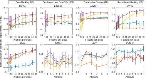
Figure 2. Improvement from RS in mean rank correlation coefficients (y-axis) of different ranking algorithms for eight datasets. In all but PubFig, our KR is comparable or better.First row:x-axis shows the number of labels per class.Second row (2–4):x-axis corresponds to the indices of attributes to learn. The absolute rank correlation coefficients including the RS results can be found in the supplemental.

and Grauman and Kovashkaet al. [20]. In general, relative attributes can be used when the labels are provided per image or object pairs. However, following Parikh and Grauman, we use the category-level labels as they facilitate objective, quantitative evaluation. For evaluation, we measure Kendall’s rank correla-tion coefficient on all inequality pairs: It counts the difference between the number of correctly ordered pairs and the number of incorrectly ordered pairs normalized by the number of total pairs.

TheETH-80dataset contains 3,280 object images from 8 different categories [23]. Each data point is represented based on the HOG (histogram of oriented gradients) descriptors as provided by Ebert et al. [10]. TheMNISTtraining dataset consists of 60,000 isolated digit images of size 28×28. We use the gray-level values as features. The cropped Street View House Numbers (SVHN) dataset contains 26,032 cropped digit images. This dataset has a similar format asMNIST; however, it exhibits large intra-class variations and includes complex photometric distortions that make the learning problem challenging [26]. Each data point is originally presented as a 32×32-sized color image. We reduced the dimensionality of the dataset to 100 using principal component analysis. The CIFAR-10dataset is a labeled subset of 80-million tiny images datasets [33]. It consists of 60,000 32×32-sized color images in 10 classes [21]. Each image in this dataset is represented based on RGB color values leading to a 3,072-dimensional vector. We applied principal component analysis to reduce

the dimensionality to 700 which contains around 99%of total variance. The Describable Textures Dataset (DTD) [7] contains 5,640 texture images arranged based on 47 manually-assigned semantic attributes (e.g.,chequeredandbumpy; 120 images per attribute). We use the semantic attribute indices as class labels.

Results. Figure 2 shows the improvement of mean rank coefficients from RankSVM (RS) with corresponding error bars (with length twice the standard deviation). Deep learning algorithm (DR) outperformed RS for all datasets demonstrating the effectiveness of deep learning for ranking problems. Also, except forPubFig, the two transductive learning algorithms TR and KR constantly outperformed RankSVM (RS). This demonstrates the effectiveness of exploiting unlabeled data in relative attribute applications. However, unlike TR and KR, performance of the model-based semi-supervised extension (SSR) is roughly on par with RS (it is better than RS onETH-80 andDTD, and worse onOSRandPubFig). Our kernel-based ranking algorithm (KR) significantly improves upon the other algorithms including the baseline transductive ranking (TR).

In particular, forMNIST, KR resulted in≈40%higher rank coefficients than other algorithms when the number of labels per class were less than 10. OnOSR, DR and KR perform best. The improvement of KR over TR is especially significant when the number of labelsl is limited. Asl increases, the performance gap between these two algorithms narrows and eventually, they become almost identical as shown in the corresponding results ofDTD.

Although the performances of KR and TR on this dataset are roughly equal, their performance variations across different attributes are significantly large. This suggests that, from the performance perspective, DR and KR are complementary. In our supplemental material, we demonstrate that by combining DR and KR we can construct a ranker that frequently outperforms other algorithms.

A notable exception to this tendency isPubFig, where DR is clear winner. This indicates that semi-supervised learning might not be always useful. One possible explanation is thatPubFig has insufficient data points to reveal the underlying manifold structure upon which the semi-supervised algorithms build (only 772 data points, while other datasets are of order thousand or ten thousand). Another explanation is simply that the data do not lie on a low-dimensional manifold. Unfortunately, verifying these possibilities is a challenging problem. Furthermore, it is not straightforward to predict which (class of) algorithms would lead to better performances on specific datasets or problems. In practice, users would interact (provide labels) with data and be able to provide feedback on theutilityof different algorithms. In this respect, the experiments demonstrate that our kernel-based ranking algorithm provides a good alternative to RankSVM and deep learning.

Hyper-parameters and time complexity. The RS, SSR, TR, and KR compared in the experiments have a regularization hyper-parameterλ. In addition, all semi-supervised learning algorithms (SSR, TR, KR) require determining theknumber of nearest neighbors and the scaling parameterσ2_{to build the graph}

Laplacian (Eq.16). We determinedσ2_{adaptively for each data}

pointx(i)such thatσ2

i becomes half of the mean distance from

x(i)to itsk-NNs [4]. The remaining hyper-parametersλandk were optimized based on a separate validation label sets which have the same size as the corresponding training set for each experiment. For DN, the number of hidden layers was fixed at 6, while the size of each layer (number of units) and the number of epochs were automatically tuned as hyper-parameters. For each run of DN, the network was trained with 5 random initializations, and the one with the smallest validation error was chosen.

The time complexity of our low-rank kernel-based ranking algorithm depends on the numbernof data points, the rank pof K factorization (Eq.21), and the knearest neighbors used to build the graph Laplacian (Eq.16). In each gradient calculation step (Eqs.23-24),BQcan be pre-calculated and QB⊤ _=−Q⊤_B⊤_{. Therefore, the most demanding} computa-tion is to calculateLBandB⊤_{[BQ]. The time complexity of} B⊤[BQ]isO(np2)whileLBtakesO(knp). In our Matlab implementation, evaluating the gradient ofBon 60,000 MNIST points withp= 50, k= 8, took≈0.004seconds on a3.6GHz machine. The time complexities of RS and TR areO(m)and

O(n), respectively withmbeing the input space dimensionality. While lower performing, RS is faster whenmis smaller than the number of data pointsn. Further, KR is less suitable for interactive applications whennis very large. That said, KR is the first algorithm that fully considers all relationships in the ordering task when designing a regularization energy.

5. Discussion and conclusion

We have empirically verified our conjecture on the effectiveness of modeling and regularizing full pairwise rank relationships with second-order tensors (kernels). Our algorithm was obtained as a discrete approximation of tensor regularization framework on manifolds. To cope with large-scale problems, we have proposed sparse factorizations. In supplemental material, we describe how our framework can be applied to learning other tensors, e.g., future work could address how to apply it to learning metric tensors.

Our low-rank factorization approach (Eq.21) was inspired by approximating the dense kernel matrix from the computational complexity perspective. Therefore, the rankpof the matrix Bwas prescribed by the expected computational and memory complexities (fixed at50throughout the entire experiments) and therefore, we haven’t actively explored the performance effect of varying rank. However, it is well known that low-rank approx-imation by itself has a regularization effect and it has been ac-tively exploited in estimating matrices, e.g., in compressed sens-ing [8], photometric stereo and structure from motion [42], and metric learning [39]. Accordingly, future work should analyze the low-rank approximation from the regularization perspective.

References

[1] A. Agresti. Analysis of Ordinal Categorical Data. Wiley-Blackwell, New Jersey, 2010.1,4

[2] G. Arvanitidis, L. K. Hansen, and S. Hauberg. Latent space oddity: on the curvature of deep generative models.

arXiv:1710.11379v2, 2018.4

[3] M. Belkin and P. Niyogi. Towards a theoretical foundation for Laplacian-based manifold methods. Journal of Computer and System Sciences, 74(8):1289–1308, 2005.1,3,5

[4] T. B¨uhler and M. Hein. Spectral clustering based on the graph p-Laplacian. InProc. ICML, pages 81–88, 2009.8

[5] O. Chapelle and S. S. Keerthi. Efficient algorithms for ranking with SVMs. Information Retrieval, 13(3):201–215, 2010.2,4

[6] O. Chapelle, B. Sch¨olkopf, and A. Zien. Semi-Supervised Learning. MIT Press, Cambridge, MA, 2010.1

[7] M. Cimpoi, S. Maji, I. Kokkinos, S. Mohamed, and A. Vedaldi. Describing textures in the wild. InProc. IEEE CVPR, pages 3606–3613, 2014.7

[8] W. Dong, G. Shi, X. Li, Y. Ma, and F. Huang. Compressive sensing via nonlocal low-rank regularization. IEEE T-IP, 23(8):3618–3632, 2014.8

[9] D. L. Donoho and C. Grimes. Hessian eigenmaps: locally linear embedding techniques for high-dimensional data. PNAS, 100(10):5591–5596, 2003.4

[10] S. Ebert, D. Larlus, and B. Schiele. Extracting structures in image collections for object recognition. InProc. ECCV, 2010.7

[11] Y. Gur. Tensor-Valued Image Regularization via Geometric Flows. PhD thesis, Tel Aviv University, 2008.1

[12] Y. Gur and N. Sochen. Regularizing flows over Lie groups. Jour-nal of Mathematical Imaging and Vision, 33(2):195–208, 2009.1

[13] M. Hein, J.-Y. Audibert, and U. von Luxburg. From graphs to manifolds - weak and strong pointwise consistency of graph Laplacians. InProc. COLT, pages 470–485, 2005.3

[14] R. Herbrich, T. Graepel, and K. Obermayer. Support vector learning for ordinal regression. InProc. IEEE ICANN, 1999.2

[15] S. C. H. Hoi and R. Jin. Semi-supervised ensemble ranking. In

Proc. AAAI, pages 634–639, 2008.5,6

[16] T. Joachims. Optimizing search engines using clickthrough data. InProc. ACM SIGKDD, pages 133–142, 2002.2

[17] J. Jost. Riemannian Geometry and Geometric Analysis. Springer, New York, 6th edition, 2011.2,3

[18] K. I. Kim. Semi-supervised learning based on joint diffusion of graph functions and laplacians. InProc. ECCV, 2016.1

[19] K. I. Kim, J. Tompkin, M. Theobald, J. Kautz, and C. Theobalt. Match graph construction for large image databases. InProc. ECCV, pages 272–285, 2012.5

[20] A. Kovashka, D. Parikh, and K. Grauman. Whittlesearch: Image search with relative attribute feedback. InProc. IEEE CVPR, pages 2973–2980, 2012.1,6,7

[21] A. Krizhevsky. Learning multiple layers of features from tiny images. Master’s thesis, University of Toronto, Canada, 2009.7

[22] J. M. Lee.Introduction to Smooth Manifolds. Springer, 2003.2,3

[23] B. Leibe and B. Schiele. Analyzing appearance and contour based methods for object categorization. InProc. IEEE CVPR, 2003.7

[24] T.-Y. Liu. Learning to Rank for Information Retrieval. Springer, Heidelberg, 2011.1

[25] Y. Liu, Y. Liu, S. Zhong, and K. C. C. Chan. Semi-supervised manifold ordinal regression for image ranking. InProc. ACM Multimedia, pages 1393–1396, 2011.1,5

[26] Y. Netzer, T. Wang, A. Coates, A. Bissacco, B. Wu, and A. Y. Ng. Reading digits in natural images with unsupervised feature learning. In Proc. NIPS Workshop on Deep Learning and Unsupervised Feature Learning, 2011.7

[27] R. S. Palais. On the differentiability of isometries. Proc. Amer. Math. Soc., 8(4):805–807, 1957.3

[28] D. Parikh and K. Grauman. Relative attributes. InProc. IEEE ICCV, pages 503–510, 2011.1,4,6

[29] F. Perbet, S. Johnson, M.-T. Pham, and B. Stenger. Human body shape estimation using a multi-resolution manifold forest. In

Proc. IEEE CVPR, pages 668–675, 2014.1

[30] M. Signoretto, Q. T. Dinh, L. D. Lathauwer, and J. A. K. Suykens. Learning with tensors: a framework based on convex optimization and spectral regularization. Machine Learning, 94(3):303–351, 2014.1

[31] M. Szummer and E. Yilmaz. Semi-supervised learning to rank with preference regularization. In Proc. ACM CIKM, pages 269–278, 2011.5,6

[32] J. B. Tenenbaum, V. Silva, and J. C. Langford. A global geometric framework for nonlinear dimensionality reduction.

Science, 290:2319–2323, 2000.1

[33] A. Torralba, R. Fergus, and W. T. Freeman. 80 million tiny images: a large data set for nonparametric object and scene recognition. IEEE T-PAMI, 30(11):1958–1970, 2008.7

[34] A. Tosi, S. Hauberg, A. Vellido, and N. D. Lawrence. Metrics for probabilistic geometries. InProc. UAI, pages 800–808, 2014.4

[35] D. Tschumperl´e and R. Deriche. Vector-valued image regulariza-tion with PDEs: a common framework for different applicaregulariza-tions.

IEEE T-PAMI, 27(4):506–517, 2005.1

[36] U. von Luxburg. A tutorial on spectral clustering. Statistics and Computing, 17(4):395–416, 2007.1

[37] K. Q. Weinberger and L. K. Saul. Distance metric learning for large margin nearest neighbor classification. JMLR, 10, 2009.1

[38] X. Yang, T. Zhang, C. Xu, S. Yan, M. S. Hossain, and A. Ghoneim. Deep relative attributes. IEEE T-MM, 18(9):1832– 1842, 2016.2,6

[39] Y. Ying, K. Huang, and C. Campbell. Sparse metric learning via smooth optimization. InNIPS, pages 2214–2222, 2009.1,8

[40] A. Yu and K. Grauman. Just noticeable differences in visual attributes. InProc. IEEE ICCV, pages 2416–2424, 2015.1

[41] J. Zhao, J. Ma, J. Tian, J. Ma, and D. Zhang. A robust method for vector field learning with application to mismatch removing. InProc. IEEE CVPR, pages 2977–2984, 2011.1

[42] Y. Zheng, G. Liu, S. Sugimoto, S. Yan, and M. Okutomi. Practical low-rank matrix approximation under robust L1-norm. InProc. IEEE CVPR, pages 1410–1417, 2012.8

[43] D. Zhou, J. Weston, A. Gretton, O. Bousquet, , and B. Sch¨olkopf. Ranking on data manifolds. InNIPS, pages 169–176, 2004.5

[44] X. Zhou and M. Belkin. Semi-supervised learning by higher order regularization. JMLR W&CP (Proc. AISTATS), pages 892–900, 2011.5