Exploring Ant Lion Optimization Algorithm to Enhance
the Choice of an Appropriate Software Reliability Growth
Model
Marrwa Abd-AlKareem Alabajee
Assist. Lecturer, Software Engineering Dept. College of Computer Sciences & Mathematics,
University of Mosul, Iraq
Taghreed Riyadh Alreffaee
Assist. Lecturer, Software Engineering Dept. College of Computer Sciences & Mathematics,
University of Mosul, Iraq
ABSTRACT
Software reliability always related to software failures, in a past few decades a software reliability growth models (SRGMs) number have been developed to predict the software reliability under different environment, but there is no single model that best fits all the real life situations and so can be recommended universally. to predict the failures of software accurately, an appropriate and best model must be chosen, this will help to estimate the cost and delivery time of the project. In this paper, Ant Lion optimization (ALO) algorithm is proposed to optimize estimation of parameters and a choice procedure is used to select an appropriate model of the software reliability that best fit available dataset of an ongoing project of the software. Employing ALO algorithm for estimating the SRGM’s parameters has provided more accurate prediction and enhance procedure of the selection, making a decision to select suitable SRGMs during the phases of the testing can be more easier to a developer of the software .The explored algorithm has been examined on various datasets of software projects and it has been noticed that this method is better than other methods proposed.
Keywords
Software Reliability, Ant Lion Optimization Algorithm, Software Reliability Growth Models.
1.
INTRODUCTION
Because of increased dependency and demand for software system, it has become necessary to develop and maintain its reliability. The system reliability drawback is that the series-parallel redundancy allocation drawback wherever either total system testing cost/effort is reduced or system dependability is maximized. Reliability isn't time dependent, is measured over execution time, so it a lot of accurately reflects system usage. when the logic path that contains a mistake is executed, Failures occur. Growth of reliability is determined as errors are detected and corrected [1]. The reliability growth models of the Software are consider One of the approaches which is used to describe the single system software behavior, failure and quantify software reliability, (SRGMs) based on data collected during testing phase. During the past 45 years, and under the analytical framework of a Non-Homogeneous Poisson Process (NHPP), many number of software reliability growth models (SRGMs) have been developed trying to integrate some realistic underlying assumptions which aim to best error detection and correction processes model.
White box and black box models are the two general classification of software reliability models (SRMs), the first one, take into consideration the software internal structure ,while the second one do not, SRGMs are considered as the black box models and are used for faults removal [2,3,4].
To obtain best model of reliability During the model selection process, there is some interests in getting the result of prediction from the model of reliability, especially SRGMs,. In order to obtain accurate and reliable selection of model, the reliability prediction must also be as accurate as possible when compared to the real data obtained. Therefore, to improve the reliability prediction, the estimation process of SRGMs parameter must also be enhanced [3].
The most important issue to the manager of the project and the developers of software engineering is the selection methodology of model, they must have a guideline in order to implement and select the suitable model of software reliability during or before the phase of testing providing no or little data on the current project [3].
In this work, we studied and explored the software reliability growth model selection methodology proposed in [5] along with the application of Ant Lion Optimizer (ALO) in parameter estimation of SRGMs. Also, two numerical examples of software reliability assessment by using the failure data in the actual software projects are shown. The results show that the use of Ant Lion Optimizer (ALO) gives better outcomes.
The paper rest is organized as follows: Section (2) reviews previous studies on reliability. Section (3) presents a brief overview of Software Reliability Growth Models. In Section (4) the Ant Lion Optimizer (ALO) are explained. Section (5) surveys the Method of selecting best SRGMs. Then, the experimental results based on two datasets are discussed in Section (6) and finally Section (7) presents the conclusion.
2.
RELATED STUDIES
In the field of software reliability, many research articles have been introduced, each of them using a different methodology leading to variations in the gained outcomes, some of these are:
Mallikharjuna and K. Anuradha [10] in 2016 investigated the improvement and application of Modified Genetic Swarm Optimization algorithm to optimize the parameters of SRGM TEF. In the same year, Alaa and Amal [11] explored the algorithm of Grey Wolf Optimization (GWO) in estimating the parameters value of SRGMs, the goal is reducing the difference between the estimated and the actual number of the software system failures. PSO was introduced in 2017 by Liang Fuh,et al. [3] to optimize a parameter estimation, distance based approach (DBA) was used to produce the selection ranking of SRGMs model. Jamal and marwah [12] estimated in the same year the parameters of SRGMs depending on Swarm Intelligence (Grey Wolf Optimizer algorithm (GWO)), This algorithm was hybrid with Real Coded Genetic Algorithm (RGA) to produced Hybrid GWO (HGWO).
3.
SOFTWARE RELIABILITY
GROWTH MODELS
The reliability growth model of the Software could be primary techniques that evaluate the software system reliability. In terms of predictability, the SRGM require intelligent performance. Any software system should afford intensive debugging and testing to control on its reliability. These processes might be expensive and need time and managers still want to true and right information related with however the reliability of the software system grows. SRGMs will estimate the initial faults amount, the reliability of the software system, the failure density, etc [1]. There are many SRGMs, but the models of Non Homogeneous Poisson process (NHPP models) is most extremely utilized, which offers more accuracy than the other models [12]. Failure count models are also referred to (NHPP) models which are based on failures number that happen in the intervals of different time. We model the discovered failures number as a stochastic process, where N(t) refer to failures number that happened at time t. when the failure intensity is not fixed then the Poisson process called non-homogenous, that means cannot be described the expected number of faults found at time (t) as a function linear in time (an ordinary Poisson process can be described by that). NHPP models suppose that the number of defects discovered during the time (t) follows (NHPP) with mean value function μ(t). mean value function derivative leads to λ(t) which is the failure density function of the software that usually decreases as faults are detected and removed [11,12].
To predict the software system reliability, A great number of NHPP models have been employed in the literature. Sixteen most commonly utilized are: Generalized Goel Model(Generalized_G)[3], Goel-Okumoto Model(Goel_O)[13], Gomperts Model(Gomperts)[3], Inflection S-Shaped Model(Inflection_S-S)[10], Logistic Growth Model(Logistic_G)[3], Modified Duane Model(Modified_D)[14], Musa Okumoto Model(Musa_O)[15], Yamada Imperfect Debugging Model1(Yamada_I_D Model1)[10], Delayed S-Shaped Model(Delayed_S-S)[11], Yamada Rayleigh Model(Yamada_R)[10], Yamada imperfect debugging Model2(Yamada_I_DModel2)[16], Yamada Exponential Model(Yamada_E)[10], P-N-Z Model(P_N_Z)[16], Pham Zhang IFD Model(Pham_Z_I)[14] ,P-Z Model(P_Z)[13] and Zhang-Teng-Pham Model(Zhang_T_P)[14].
4.
ANT LION OPTIMIZER
4.1
Inspiration
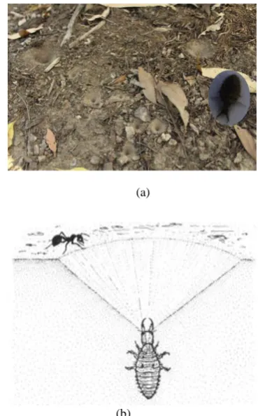
Antlions belong to the Myrmelentidae family, a group of insects. The major stages of the antlions lifecycle are: Larval and adult phase, first one named "doodlebug", because antlion leaves the trails in the sand while searching for a perfect place to construct its snare. Fig. 1 (a) show the hunting operation when the antlion creates in the soft sand funnel pits, then it waits at the pit's bottom. In a Fig. 1(b) Show sliding to the pit's bottom, the antlion is directly seized the prey, it throws sands towards the pit's edge to make the prey slides into the pit's bottom, if this prey tries to get-away from the snare, the larva also undermines the pit's sides, this lead it to fall and fetch the prey with them [17][18]. The name of the antlion comes from their unique behavior of the hunting. It makes a circular path when moving, and by using its massive jaw, the sands is thrown ,leading to a cone-shaped pit in the sand[18]. ALO algorithm's Inspiration comes from the antlion’s larvae behavior[18].
(a)
[image:2.595.340.525.287.584.2](b)
Fig. 1 the hunting process and behavior of antlion
4.2
ALO Algorithm Operators
The algorithm of Antlion Optimization Algorithm (ALO) simulate interaction between ants in the snare and antlions, to exemplify this interactions, ants are wanted to move over the space of the search, and antlions are allowed to hunt them and become fitter using traps. in nature, ant's movement become randomly when looking-for the food, to modeling such movement, the equation of random walk is [19]:
...(1)
Where:
t: represent the iteration .
r(t): stochastic function defined as follows[19]:
……… (2)
Where:
rand: a random number created in the period of [0,1].
The ants position (variables of all solutions) are stored and using through optimization in the matrix below [18]:
..……… (3)
Where:
MAnt: the matrix contains the position of each ant.
n: the ants number . d:the variables number [19].
It should be noted that individuals in GA or particles in PSO are similar to ants. The ant's position represents parameters for a particular solution. the fitness function is used during optimization For evaluating each ant, this fitness value stores in the following matrix ( MOA)[18]:
…………. (4)
In addition to ants, the positions and fitness values of the antlions are also save in the MAntlion and MOAl matrices [20]
[18] .
4.2.1
Ant's Random walks
All Random walks are based on Eq. (1) ,with random walks, Ants position are updated at every step of optimization, however, Eq. (1) cannot be directly used for updating position of ants [18]. To keep ants' random walks inside the space of the search, they are normalized utilizing the equation below [17]:
………...….. (5) Where:
ai: the minimum of random walk of i-th variable.
bi: the maximum of random walk in i-th variable. : the minimum of i-th variable at t-th iteration.
indicates the maximum of i-th variable at t-th iteration.
To ensure the occurrence of random walks inside the space of the search, The above equation should be applied in each iteration [18] .
4.2.2
Trapping in antlion’s pits
Ants' random walks are influenced by the snares of the antlion. In order to represent this mechanism mathematically, the equations below are proposed [21][18]:
……… (6)
……… (7)
Where:
Ct: the minimum of all variables at t-th iteration.
dt: : vector including the maximum of all variables at t-th iteration.
Cti: the minimum of all variables for i-th ant.
dti :the maximum of all variables for i-th ant.
Antlionttj: the position of the selected j-th antlion at t-th
iteration.
4.2.3
Building trap
To model the capability of hunting of the antlions during optimization, we use the selection of roulette wheel for choose antlions based on their fitness. This assumption gives high opportunity to the fitter antlions for catching ants[18].
4.2.4
Sliding ants towards ant lion
Proportional to Antlion's' fitness, they are able to build traps and ants need to randomly move. However, the antlions throwing sands outwards the pit's center, when they realize that the prey (ant) is fell into the trap. With This action the trapped ant slips down while is attempting to escape. To modelling this behavior mathematically, the radius of ants' random walks hyper-sphere is decreased adaptively. in this regard, The following equations are proposed [21][22]:-
……… (8)
= ………..… (9)
Where:
I: is a ratio, calculate as[17]:
………..………. (10)
Where:
t: the present iteration.
T: the iterations maximum number .
w: a constant defined based on the present iteration (w = 2 when t > 0.1T, w = 3 when t > 0.5T, w = 4 when t > 0.75T, w = 5 when t > 0.9T, and w = 6 when t > 0.95T)[18].
4.2.5
seizuring prey and re-constructing the pit
The antlion’s jaw caught the ant when the ant arrives the pit's bottom .This is final stage of hunt, the antlion, After that, consumes the body of the ant, when it pulls the ant inside the sand. For simulating this process, it is supposed that, when an ant becomes fitter (goes inside sand) than its corresponding antlion, catching prey occur. To boost the chance of antlions to capturing new prey, the position of antlion must be updated to the latest position of the hunted ant. The equation below is explain this state [18]:
…… (11) Where:
t: the present iteration.
: symbolize the position of selected j-th antlion at t-th iteration.
: indicate the position of i-th ant at t-th iteration.
4.2.6
Elitism
The evolutionary algorithms have a feature called Elitism that allows at any phase of optimization procedure to choose the better solution(s). an elite is considered as the best antlion (fittest one) obtained and saved in each iteration, an elite should be able to influence of all the ants' movements during iterations. Therefore, it is supposed that each ant walks randomly around the antlion selected by the roulette wheel and the elite simultaneously, as following below [18][22]:
4.3
ALO Algorithm
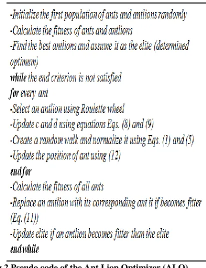
[image:4.595.78.284.121.389.2]The ALO algorithm steps can be summarized as shown in Fig.2 [18]:
Fig.2 Pseudo code of the Ant Lion Optimizer (ALO)
5.
METHOD OF SELECTING BEST
SRGMs
The method which is used in this paper for select the best model of software reliability from SRGMs group proposed in [5] with some modification, the steps of this method are: 1- During the testing process, a record of the periodic of the
detected failures' cumulative number until the test date is maintained.
2- find the best value of parameters of the SRGMs probable group by applying Ant Lion Optimization algorithm (ALO), and later compute the following criteria for all models:
Rsq: it is used to assess the model fit to the available data. RMSE: its measures the differences between values predicted by a model and the values actually observed.
3- check the Rsq and RMSE value for all the models probable group and select them for which:
specified value ………. (13) And
specified value …….. (14)
According to the value of criterion of the dataset, The (specified value) is chosen.
4- For each models that meet the two criteria previously,
compute from formula 15:
……….. (15), Where:
: The present value of failures' predicted number utilizing the model chosen.
: The observed actual failures in the dataset.
5- After that, for each of the selected models, calculate the total number of expected failures 'a' and remaining failures 'a-m(t)' and the estimated time by which 95% confidence limit using formula 16:
….. (16) Where:
: the failures' estimates number that detected until date (m(t))
ACR: the failures' actual number discovered till date (m(t)). 6- the best fit model is the model whose value of EST
closest to one. By utilizing computed data, the formula 17 used to arrange the models:
.... (17)
Where:
.
: Amongst all the values of for selected models, is the least value.
Is the value for that specific model.
7- Choose the suitable model for the data that gives best future predictions from the top ranked models.
6.
EXPERIMENTAL RESULTS
In this work, we develop the technique proposed in[5] for solving the problem of choice the best software reliability growth model Which fits to certain dataset, we used an ant lion algorithm to estimating the parameters of the selected SRGMs instead of using a software in MATLAB for curve fitting. Firstly we set the search agents (ant lions) number and the iterations' maximum number for the experiment. By tuning these two parameters in experiment, we observed that (40) agents and (1000) iterations give highly acceptable outcomes. In Our experiments we used two dataset of software projects to explore the use of ant lion algorithm and to estimate the parameters of sixteen SRGMs that selected in this work and then apply the steps of technique in [5] to choice best SRGMs that best fit to selected dataset.
6.1
Case Study1
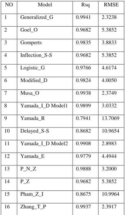
The first dataset is DS1 presented in [23], is relied upon as the first case study with an hour data collected, it includes failures' number and the failures' cumulative number since the starting of test is recorded for each hour. The total observed number of failures is 136 within 25 hours. We apply the ant lion algorithm to estimate the parameters values of the selected models, the Table (1) display the value of parameters estimated using ALO for DS1. and then compute the Rsq and RMSE for DS1, Table (2) shows the values of Rsq and RMSE for DS1. Later We compare the Rsq and RMSE values of the models selected with a specific value according to
Table (1)the value of parameters estimated using ALO for DS1
NO Model Parameter Values
1 Generalized_G a=180.1464, b=0.1733, c=0.6578 2 Goel_O a=136.3067, b=0.1375
4 Inflection_S-S a=136.2938, b=0.1376, β=0.9101*10^(-3)
5 Logistic_G a=136.2275, b=0.1901, k=2.6706 6 Modified_D a=160.1429, b=11.8145, k=1.6057 7 Musa_O a=46.1497, b= 0.7428
8 Yamada_I_D Model1
a=87.3959, b= 0.3148, c=0.0220
9 Yamada_R a=205.2624, b= 0.8857, c=0.0467 10 Delayed_S-S a=124.9183, b=0.3623
11 Yamada_I_D Model2
a=88.2191, b= 0.2766, c =0.0271
12 Yamada_E a=167.8129,α =1.9806,β =0.0630 13 P_N_Z a=71.3325,b=0.6397,α=0.0420,
β=0.7693
14 P_Z a=10.4939, b= 0.1375, c=125.8155, α =42042.5087, β= 0.1311*10^(-3)
15 Pham_Z_I a=124.8617, b=0.3521, d=0.2757*10^(-3)
16 Zhang_T_P a=77.7118, b=0.0698, c= 0.0768, α = 0.5354, β=0.4865
equations(13,14), the specified value chosen as (0.95) for equation(13) because most of the criterion values of the models are good and close to one, and chosen as(10) for equation (14). From table (2) we conclude that Yamada Rayleigh (Yamada_R), Delayed S-shaped (Delayed_S-S) and Pham Zhang IFD (Pham_Z_I) models do not subject to the two preceding conditions in equation (13,14), So it will be neglected. For all Other models that are subject to the previous two conditions, we calculate the value of PRED from equation (15). After that we calculated the values of EST from equation(16) for time (5,10,15,20) Using computed data, models may be ranked by applying equation(17), then we choose appropriate model from amongst the top models ranked, the Generalized_Goel model (Generalized_G) is gives best future prediction for all times as shown in table(3). Fig. 3 show the curve of the actual accumulated failures and the estimated accumulated failures of Generalized_G for DS1.
6.2
Case Study 2
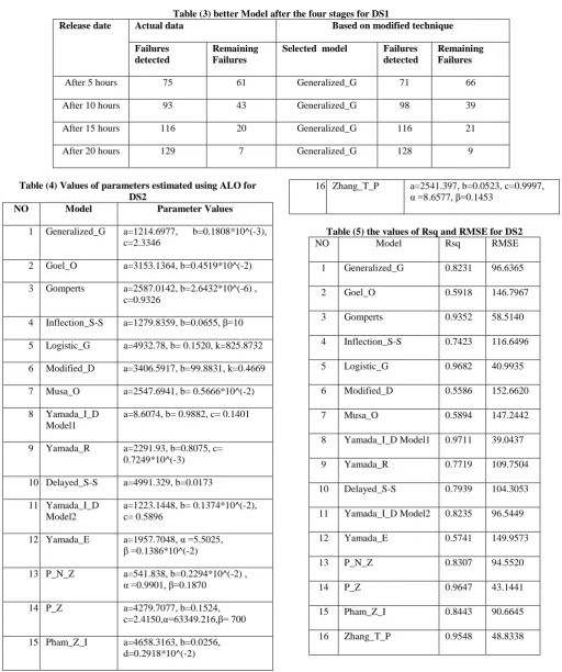
In the second case study, we used DS2 that including 34 measurements as presented in [24]. Its include the failures'
Table (2) the values of RSQ and RMSE for DS1
NO Model Rsq RMSE
1 Generalized_G 0.9941 2.3238
2 Goel_O 0.9682 5.3852
3 Gomperts 0.9835 3.8833
4 Inflection_S-S 0.9682 5.3852 5 Logistic_G 0.9766 4.6174 6 Modified_D 0.9824 4.0050
7 Musa_O 0.9938 2.3749
8 Yamada_I_D Model1 0.9899 3.0332
9 Yamada_R 0.7941 13.7069
10 Delayed_S-S 0.8682 10.9654 11 Yamada_I_D Model2 0.9908 2.8983
12 Yamada_E 0.9779 4.4944
13 P_N_Z 0.9888 3.2000
14 P_Z 0.9682 5.3852
15 Pham_Z_I 0.8675 10.9964
16 Zhang_T_P 0.9937 2.3917
[image:5.595.44.290.67.425.2] [image:5.595.325.532.91.446.2]Table (3) better Model after the four stages for DS1
Release date Actual data Based on modified technique Failures
detected
Remaining Failures
Selected model Failures detected
Remaining Failures
After 5 hours 75 61 Generalized_G 71 66
After 10 hours 93 43 Generalized_G 98 39
After 15 hours 116 20 Generalized_G 116 21
After 20 hours 129 7 Generalized_G 128 9
Table (4) Values of parameters estimated using ALO for DS2
NO Model Parameter Values
1 Generalized_G a=1214.6977, b=0.1808*10^(-3), c=2.3346
2 Goel_O a=3153.1364, b=0.4519*10^(-2) 3 Gomperts a=2587.0142, b=2.6432*10^(-6) ,
c=0.9326
4 Inflection_S-S a=1279.8359, b=0.0655, β=10 5 Logistic_G a=4932.78, b= 0.1520, k=825.8732 6 Modified_D a=3406.5917, b=99.8831, k=0.4669 7 Musa_O a=2547.6941, b= 0.5666*10^(-2) 8 Yamada_I_D
Model1
a=8.6074, b= 0.9882, c= 0.1401
9 Yamada_R a=2291.93, b=0.8075, c= 0.7249*10^(-3)
10 Delayed_S-S a=4991.329, b=0.0173 11 Yamada_I_D
Model2
a=1223.1448, b= 0.1374*10^(-2), c= 0.5896
12 Yamada_E a=1957.7048, α =5.5025, β =0.1386*10^(-2)
13 P_N_Z a=541.838, b=0.2294*10^(-2) , α =0.9901, β=0.1870
14 P_Z a=4279.7077, b=0.1524, c=2.4150,α=63349.216,β= 700 15 Pham_Z_I a=4658.3163, b=0.0256,
d=0.2918*10^(-2)
16 Zhang_T_P a=2541.397, b=0.0523, c=0.9997, α =8.6577, β=0.1453
Table (5) the values of Rsq and RMSE for DS2
NO Model Rsq RMSE
1 Generalized_G 0.8231 96.6365
2 Goel_O 0.5918 146.7967
3 Gomperts 0.9352 58.5140
4 Inflection_S-S 0.7423 116.6496 5 Logistic_G 0.9682 40.9935 6 Modified_D 0.5586 152.6620
7 Musa_O 0.5894 147.2442
8 Yamada_I_D Model1 0.9711 39.0437
9 Yamada_R 0.7719 109.7504
10 Delayed_S-S 0.7939 104.3053 11 Yamada_I_D Model2 0.8235 96.5449
12 Yamada_E 0.5741 149.9573
13 P_N_Z 0.8307 94.5520
14 P_Z 0.9647 43.1441
15 Pham_Z_I 0.8443 90.6645
[image:6.595.41.554.65.678.2]Table (6) better Model after the six stages for DS2
Release date Actual data Based on modified technique Failure
detected
Remaining Failure
Selected model Failure detected
Remaining Failure
After 5 weeks 43 806 Yamada I_ D Model1 15 868
After 10 weeks 70 779 Yamada I_ D Model1 31 852
After 15 weeks 91 758 Yamada I_ D Model1 62 821
After 20 weeks 105 744 Yamada I_ D Model1 124 759
After 25 weeks 249 600 Yamada I_ D Model1 250 633
After 30 weeks 405 444 Yamada I_ D Model1 504 379
Fig.(3) The Curve of the Actual Accumulated Failures and the Estimated Accumulated Failures of Generalized_G for DS1
Fig. 4 The Actual and Estimated Accumulated Failures Curves for Yamada I_ D Model1 for DS2
7.
CONCLUSION
In this paper, the problem of choosing the best software reliability growth model for a particular dataset was discussed. Sixteen software reliability growth models were applied on the failure data and the Ant Lion Optimizer algorithm was utilized to estimate the selected models parameters. The quantifiable parameters are used to predict the cumulative failure of the software system. Then a set of procedure was applied to sort the models from the best to the
least suitable for the data. The results confirm the effectiveness of the ALO to resolve the issue of estimate the SRGMs parameters, this leads to a good choice of the best model for proper data.
8.
REFERENCES
[1] Diwaker, C. and Goyat, S. 2014. Parameter Estimation of Software Reliability Growth Models Using Simulated Annealing Method, International Journal of Computer Applications Technology and Research Volume (3), Issue (6), pp:377 - 380.
0 20 40 60 80 100 120 140 160
1 3 5 7 9 11 13 15 17 19 21 23 25
Actual data Estimated data
Numb
er
o
f
fa
ilu
res
Time(Hour)
0 200 400 600 800 1000
1 3 5 7 9 11 13 15 17 19 21 23 25 27 29 31 33 Actual data
Estimated data
Time (weeks)
N
u
mbe
r
o
f fa
ilu
re
[image:7.595.76.518.87.601.2][2] Al Turk, L. I. and Alsolami, E. G. 2016. JELINSKI-MORANDA SOFTWARE RELIABILITY GROWTH
MODEL: A BRIEF LITERATURE AND
MODIFICATION, International Journal of Software Engineering & Applications (IJSEA), Vol.( 7), No.(2). [3] ONG, L. F., ISA, M. A., JAWAWI, D. N. A. and
ABDUL HALIM, S. 2017. Improving software reliability growth model selection ranking using particle swarm optimization, Journal of Theoretical and Applied Information Technology, 15th January 2017,Vol.(95), No.(1) .
[4] Iqbal, J. 2016. Analysis of Some Software Reliability Growth Models with Learning Effects, I.J. Mathematical Sciences and Computing, 2016, 3, pp:58-70, Published Online July 2016 in MECS (http://www.mecs-press.net) DOI: 10.5815/ijmsc.2016.03.06.
[5] Miglani, N. 2014. On the Choice of an Appropriate Software Reliability Growth Model, International Journal of Computer Applications (0975 – 8887) Volume (87), No.(9).
[6] Hsu, C. J. and Huang, C.Y. 2010. A Study on the Applicability of Modified Genetic Algorithms for the Parameter Estimation of Software Reliability Modeling, IEEE 34th Annual Computer Software and Applications Conference, pp:531-540.
[7] Shanmugam, L. and Florence, L. 2012. Comparison of Parameter Best Estimation Method for Software Reliablity Models, International Journal of Software Engineering & Applications (IJSEA).
[8] AL-Saati, N. A. and Abd-AlKareem M. 2013. The Use of Cuckoo Search in Estimating the Parameters of Software Reliability Growth Models,(IJCSIS) International Journal of Computer Science and Information Security, Vol. (11), No.(6).
[9] Diwaker, C. and Goyat, S. 2014. Parameter Estimation of Software Reliability Growth Models Using Simulated Annealing Method, International Journal of Computer Applications Technology and Research, Volume (3), Issue (6), pp:377 – 380.
[10]Mallikharjuna Rao K. and Anuradha, K. 2016 . A New Method to Optimize the Reliability of Software Reliability Growth Models using Modified Genetic Swarm Optimization, International Journal of Computer Applications (0975 – 8887), Volume (145), No.(5). [11]Sheta, A. F. and Abdel-Raouf, A. 2016. Estimating the
Parameters of Software Reliability Growth Models Using the Grey Wolf Optimization Algorithm, (IJACSA) International Journal of Advanced Computer Science and Applications, Vol.(7), No.(4).
[12]Alneamy, J. S. M. and Dabdoob, M. M. A. 2017. The Use of Original and Hybrid Grey Wolf Optimizer in Estimating the Parameters of Software Reliability
Growth Models, International Journal of Computer Applications (0975 – 8887), Volume (167) , No.(3). [13]Song,K. Y., Chang, I. H. and Pham, H. 2017. An NHPP
Software Reliability Model with S-Shaped Growth Curve Subject to Random Operating Environments and Optimal Release Time, Applied Sciences, 2017, 7, 1304; doi:10.3390/ app7121304.
[14]Kaur, R. and Panwar, p. 2015. Study of Perfect and Imperfect Debugging NHPP SRGMs used for Prediction of Faults in a Software, IJCSC, Vol. (6), No. (1),pp:73-78.
[15]Aggarwal, G. and Gupta, V. K. 2014. Software Reliability Growth Model, International Journal of Advanced Research in Computer Science and Software Engineering, Volume(4), Issue (1).
[16]Singh, M. and Bansal, V. 2015. Parameter Estimation and Validation Testing Procedures for Software Reliability Growth Model, International Journal of Science and Research (IJSR), Volume (5), Issue(12). [17]Petrović, M., Petronijević, J., Mitić, M., Vuković, N.,
Plemić, A., Miljković, Z. and Babić, B. 2015. The Ant Lion Optimization Algorithm For Flexible Process Planning, journal of production engineering, vol .( 18),No.(2).
[18]Mirjalili, S. 2015. The Ant Lion Optimizer, Advances in Engineering Software, 83 (2015), pp: 80–98.
[19]Satheeshkumar, R. and Shivakumar, R. 2016. Ant Lion Optimization Approach for Load Frequency Control of Multi-Area Interconnected Power Systems, journal of scientific research publishing, 7, 2357-2383.
[20]Talatahari, S. 2016. Optimum Design Of Skeletal Structures Using Ant Lion Optimizer, International Journal Of Optimization In Civil Engineering, 6(1),pp:13-25.
[21]Nischal, M. M. and Mehta, S. 2015. Optimal Load Dispatch Using Ant Lion Optimization, Int. Journal of Engineering Research and Applications, ISSN: 2248-9622, Vol.(5), Issue(8), (Part - 2) August 2015, pp.10-19. [22]Ali, E. S., Abd Elazima, S. M. and Abdelaziz, A. Y. 2017. Ant Lion Optimization Algorithm for optimal location and sizing of renewable distributed generations, Renewable Energy, Vol.(101) pp:1311-1324.
[23]Mohd, R. and Nazir, M. 2012. Software Reliability Growth Models: Overview and Applications, Journal of Emerging Trends in Computing and Information Sciences, VOL. (3), NO. (9).