Volume 177 – No. 8, October 2019
Phased Bee Colony Optimization Algorithm for Solving
Mathematical Function
Rahul Kumar Mishra
Enterprise Solutions Supply Chain Tata Consultancy Services
New Delhi, India
ABSTRACT
In this article, we have proposed an efficient Bee Colony
Optimization method, namely Phased Bee Colony
Optimization (PBCO) technique for solving mathematical functions in a multidimensional space. The search process of the optimization approach is directed towards a region or a hypercube in a multidimensional space to find a global optimum or near global optimum after a predefined number of iterations. The process in the entire search area to another region (new search area) surrounding the optimum value found so far after a few iterations and restarts the search process in the new region. However, the search area of the new region is reduced compared to previous search area. Thus, the search process finding advances and jumps to a new search space (with reduced area space) in several phases until the algorithm is terminated. The PBCO technique has tested on a set of mathematical benchmark functions with number of dimensions up to 100 and compared with several relevant optimizing approaches to evaluate the performance of the algorithm. It has observed that the proposed technique performs either better or similar to the performance of other optimization methods.
Keywords
Bee Colony Optimization; phased; optimization; hypercube; mathematical functions
1.
INTRODUCTION
The Artificial Bee Colony (ABC) method is a metaheuristic population based evolutionary search algorithm for solving various optimization problems. The algorithm is inspired by the intelligent foraging behavior of honeybee swarms in nature. The ABC algorithm basically imitates the behavior of real bees searching for food. The ABC produces new solution according to the stochastic variance process. It is an iterative algorithm in which the magnitudes of the perturbation are important for finding new solution. The ABC has been applied for solving different problems like scheduling, timetabling, travelling salesman problem, data mining and clustering and many more. Apart from these, the researchers have always made an attempt to enhance the performance of the ABC optimization with or without hybridization for solving problems in discrete as well as continuous domains. Pham and Castellani [1] proposed a continuous exploitative neighborhood search process combined with random explorative search, for increasing the speed and accuracy of the optimization method. Zou, Chen and Zhang [2] had
developed an improved ABC algorithm to solve
multiobjective optimization problems. Akbari, Mohammadi and Ziarati [3] developed a novel bee swarm optimization algorithm to solve numerical function optimization. Aydin, Liao, Oca and Stutzle [4] modified the ABC by making the population growth over time to improve the performance of algorithm. Zhang [5] used this algorithm to solve the job shop
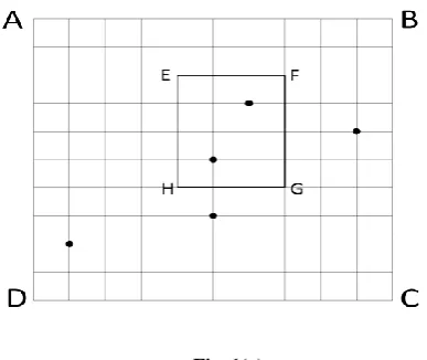
scheduling problem. Yildih [6] proposed an approach with ABC algorithm for optimal selection of cutting parameters in multipass turning operation. Karaboga and Ozturk [7] applied ABC technique in the application of clustering.We have proposed a new technique based on the ABC algorithm for solving mathematical optimization problems in both discrete and continuous domains. The name of proposed algorithm is Phased Bee Colony Optimization (PBCO). The search in PBCO advances in multiple phases depending on the quality of nectar in the flower patches in a particular region of search space where the best quality of nectar till found after the end of a few number of iterations in each phase. In PBCO the search always jumps to a new region (i.e. the neighboring hypercube in a multidimensional space) with same number of bees. However, the space of new search area is smaller than the previous (hypercubic) search area as shown in Fig. 1. The reduction of search space is done along all dimensions. We have compared our proposed method with some relevant optimization techniques testing on a set of standard benchmark functions with problem dimensions upto 100. The rest of the paper is organized as follows. Section II describes the algorithms of simple ABC and PBCO techniques. It also discusses the search space partitioning process with progress of search. The experimental results along with discussion are provided in Section III. Section IV concludes the paper.
2.
FUNCTION OPTIMIZATION USING
ABC
A global optimization problem can generally be formulated as a pair (S, f) where S ⊆ Rn is a bounded set on Rn and f: S
⟼ R is an n- dimensional real- valued function. The objective of the problem is to find a point opt ∈ S on Rn
such that (xt)
is a global optimum on S. We have to find xt ∈ S according to
the following equations for minimization or maximization problems, respectively:
∀x ⊆ s ∶ (xt) f x
∀x ⊆ s ∶ (xt) f x
where f may not be a continuous function but it must be bounded.
2.1
Conventional ABC Algorithm
Volume 177 – No. 8, October 2019
has done. Onlooker bee’s tries to select possibly the best food sources from those discovered by the employed bees, and then further search for foods around the selected food source. Bees whose food sources get abandoned got changed from employed bees to Scout bees, assigned with new random food source [8, 9, and 10]. The simple ABC is a global optimization method, which used for solving various optimization problems [1 – 7]. The ABC algorithm represented algorithmically as follows.
1. Initialize the population of solutions (Xi,j) in search
space and , here denotes lower limit and upper limit of search space and i,j here denotes lower limit and upper limit of search space.
2. Evaluate the population
3. Repeat
4. Produce new solutions (Ui,j) in the neighborhood of
Xi,j and evaluate.Ui,j = Xi,j+ Oi,j (Xi,j – Xk,j) , where
k= solution in the neighborhood of I andO= random number in the range [-1,1].
5. Greedy selection process will be applied in the selection between Xi,j and Ui,j .
6. Calculate value ( of solutions followed by the calculation of probability ( where
7. Greedy selection is again applied and the abandoned solution is determined, if exists and it is replaced by the new randomly produced solution.
8. Memorize the best food source found so far until
requirements has met.
9. Stop
2.2
Optimization using PBCO
We have modified the simple ABC technique into a phased ABC approach by directing the search towards the area where the possibility of best result is maximum and reducing the search space accordig to the user’s choice. The repetitive reduction of the search area in a 2-D space is described in the following section. Initially, the PBCO algorithm starts searching to find the optimum value in the entire search space. The search process then runs for a certain number of iterations (say, Ik) and gives the best possible
solutions after the completion of Ik iterations. The search
process is directed towards the area where closed to optimum solution is reached after a few iterations in each phase. The PBCO iterates executes iteratively in multiple phases and in each phase, we find the area i n which the best optimum value lies. The search space is reduced to corresponding area along all dimensions. Once the optimization methods completes Ik the best solution and the position of that
solution is also calculated in the search space. The space where the best solution is achieved is reduced along all dimensions (discussed in detail in Section II C). The bee population is regenerated in that reduced search space. The PBCO approach restarts in the new search area and continues again for Ik times before it is transferred to another
new search space considering the best solution approaching
the optimum. The PBCO finally terminates after the completion of Imax iterations.
Algorithmic representation of the PABC technique
1. Initialize the population of bees, other parameters and iteration I=1.
2. Create solutions for all bees.
3. Find the area where the best solution lies of current phase.
4. Redefine the search space surrounding the area where the
best solution achieved and regenerate the population of bees following the elitist model.
5. Move the search to the new search space (See Fig. 1) which is smaller in size than the previous search space and restart the search process.
6. Increment I= I + Ik . If I ≤ Imax, then go to step 2.
7. Stop.
2.3
Search space reduction and
transferring of the PBCO method
Volume 177 – No. 8, October 2019
Fig. 1(a)
Partitioning of space and best solution of first five iterations (1-5) at phase 1.
Fig. 1(b)
Partitioning newly defined search space and best solutions of next five iterations at phase 2.
Best solution of last five iterations and extraction of global or near-global optimum solution at final stage.
[image:3.595.63.257.75.238.2]Fig. 1(c)
Fig. 1 Reduction of search space and transferring of the PBCO technique in 3 phases.
3.
EXPERIMENTAL STUDIES
The performance of the PBCO technique on a set of 20 mathematical functions evaluated in two parts. In the first part, we have compared the results of PBCO with several other relevant optimization algorithms to establish it as an efficient optimization algorithm. In the second part, we have optimized functions F2 – F15 to show the effectiveness of the
proposed method in optimizing problems with higher dimensions (up to 100). We have considered the set of 20 standard benchmark functions taken from [20], which has listed in Table 1. The results of the optimization methods except the PBCO in Table 3 have also taken from [20]. The functions F1 – F20 are a combination of unimodal and
multimodal functions. The functions F16 – F20 are low
dimensional compared to other functions (F1 – F15) (see
Tables 1 and 2). Table 2 depicts the basic parameters of the tested functions (F1 – F20).
3.1
Parameter Setup.
[image:3.595.63.264.283.455.2]In the experiment, we have considered that the population size of bees is µ (= 50) until the end of the proposed optimization algorithm. For each function in Table 1, the algorithm PBCO ran 50 times and the average of the optimum results of 50 runs tabulated in Table 3 for the PBCO method. The dimension of the function has denoted by n as described in Table 2 for each function. We have run the PBCO technique for I iterations to calculate the optimum value in each phase (hypercube) for directing the search in redefined search space for the next phase. The new search space is generated by reducing u% of the length along all dimensions of the previous search space (see Figs. 1(a) – 1(c)). For all tested functions in Table 1, we have considered the value of I to be 10 and the value of u is set to 25. If the value of I is increased towards the higher side of the range, the search process slows down i.e. more number of iterations are required to converge (by the algorithm). On the other hand, if u is set to a high value (more than 25), the algorithm (PBCO) may not converge to a global or near – global optimum solution since the optimization method may have the possibility to miss the global or near – global optimum due to fast reduction of the search space after repetitive I iterations. In the experiment, we have tried to maintain the values of I and u within the range such that the PBCO approach converges faster to the global optimum for all the functions in Table 1.
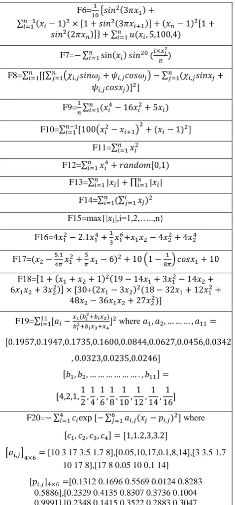
Table 1. Functions tested for optimization
F1= F2=
F3=
F4=
F5=
where
and
[image:3.595.64.260.541.711.2] [image:3.595.308.546.557.769.2]
Volume 177 – No. 8, October 2019
F6=
F7=
F8=
F9=
F10=
F11=
F12=
F13=
[image:4.595.49.288.70.583.2] [image:4.595.315.541.342.762.2]F14=
F15=max{| |,i=1,2,…..,n}
F16= F17=
F18=
+
F19= where
F20= where
[10 3 17 3.5 1.7 8],[0.05,10,17,0.1,8,14],[3 3.5 1.7
10 17 8],[17 8 0.05 10 0.1 14]
[0.1312 0.1696 0.5569 0.0124 0.8283
0.5886],[0.2329 0.4135 0.8307 0.3736 0.1004 0.9991],[0.2348 0.1415 0.3522 0.2883 0.3047 0.6650],[0.4047 0.8828 0.8732 0.5743 0.1091 0.0381]
Table 2. Basic parameters of the tested functions
Func. Search Space Dimension(n) Optimal value
F1 [-500,500]n 30 -12569.5
F2 [-5.12,5.12]n 30 0
F3 [-32,32]n 30 0
F4 [-600,600]n 30 0
F5 [-50,50]n 30 0
F6 [-50,50]n 30 0
F7 [0,π]n 100 -99.2784
F8 [-π,π]n 100 0
F9 [-5,5]n 100 -78.33236
F10 [-5,10]n 100 0
F11 [-100,100]n 30 0
F12 [-1.28,1.28]n 30 0
F13 [-10,10]n 30 0
F14 [-100,100]n 30 0
F15 [-100,100]n 30 0
F16 [-5,5]n 2 -1.0316285
F17 [-5,10],[0,15] 2 0.398
F18 [-2,2]n 2 3
F19 [-5,-5]n 4 0.0003075
F20 [0,1]n 6 -3.32
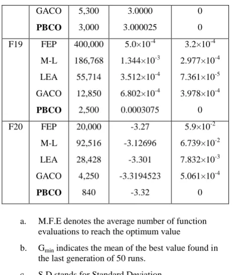
Table 3. Comparative results of PBCO with relevant optimization algorithms
Fun. Algo. M.F.E Gmin S.D
F1 ALEP
FEP
OGA/Q
M-L
LEA
GACO
PBCO
150,000
900,000
302,116
655,895
287,365
8300
3900
-11469.2
-12554.5
-12569.453
-5461.826
-12569.454
-12569.48
-12569.48
58.2
52.6
6.447×10⁻⁴
275.15
4.831×10⁻⁴
1.953×10⁻²
1.126×10⁻⁴
F2 ALEP
FEP
OGA/Q
M-L
LEA
GACO
PBCO
150,000
500,000
224,710
305,899
223,803
19,650
4,480
5.85
4.6×10⁻²
0
121.7575
2.103×10⁻¹⁸
0
1.19080×10⁻¹⁴
2.07
1.2×10⁻²
0
7.7572
3.359×10⁻¹⁸
0
1.191×10⁻¹⁴
F3 ALEP
FEP
OGA/Q
M-L
LEA
GACO
PBCO
150,000
150,000
112,421
121,435
105,926
30,550
6,325
1.9×10⁻²
1.8×10⁻²
4.440×10⁻¹⁶
2.5993
3.274×10⁻¹⁶
3.641×10⁻¹⁴
6.32397×10⁻¹²
1.0×10⁻³
2.1×10⁻²
3.989×10⁻¹⁷
9.425×10⁻²
3.001×10⁻¹⁷
4.47×10⁻¹⁴
3.236×10⁻¹⁴
F4 ALEP
FEP
OGA/Q
150,000
200,000
134,000
2.4×10⁻²
1.6×10⁻²
0
2.8×10⁻²
2.2×10⁻²
Volume 177 – No. 8, October 2019 M-L LEA GACO PBCO 151,281 130,498 9,950 4,475 1.1894×10⁻¹ 6.104×10⁻¹⁶ 0 3.08999×10⁻¹² 1.040×10⁻² 2.513×10⁻¹⁷ 1.1841×10⁻² 1.598×10⁻¹⁴
F5 ALEP
FEP OGA/Q M-L LEA GACO PBCO 150,000 150,000 134,556 146,209 132,642 16,900 6,175 6.0×10⁻⁶ 9.2×10⁻⁶ 6.019×10⁻⁶ 2.105×10⁻¹ 2.482×10⁻⁶ 1.571×10⁻³² 2.65491×10⁻¹⁶ 1.0×10⁻⁶ 3.6×10⁻⁶ 1.159×10⁻⁶ 3.609×10⁻² 2.276×10⁻⁶ 1.570×10⁻³² 2.655×10⁻¹⁶
F6 ALEP
FEP OGA/Q M-L LEA GACO PBCO 150,000 150,000 134,143 147,928 130,213 18,550 8,670 9.8×10⁻⁵ 1.6×10⁻⁴ 1.869×10⁻⁴ 1.50534 1.734×10⁻⁴ 1.3497×10⁻³² 8.2983×10⁻¹⁵ 1.2×10⁻⁵ 7.3×10⁻⁵ 2.615×10⁻⁵ 2.25564 1.205×10⁻⁴ 1.350×10⁻³² 8.298×10⁻¹⁵
F7 OGA/Q
M-L LEA GACO PBCO 302,773 329,087 289,863 9,250 3,975 -92.83 -23.97544 -93.01 -99.26889 -99.26889 2.626×10⁻² 6.2875×10⁻¹ 2.314×10⁻² 6.279×10⁻¹ 2.165×10⁻²
F8 OGA/Q
M-L LEA GACO PBCO 190,031 221,547 189,427 3,350 1,580 4.672×10⁻⁷ 2.58778×10⁴ 1.627×10⁻⁶ 1.7886×10⁻⁷ 3.341×10⁻¹⁰ 1.293×10⁻⁷ 1.73975×10³ 6.527×10⁻⁷ 2.38×10⁻⁷ 1.42×10⁻¹⁰
F9 OGA/Q
M-L LEA GACO PBCO 245,930 251,199 243,895 8,550 3,750 -78.300029 -35.80995 -78.310 -78.332275 -78.33233 6.288×10⁻³ 8.9146×10⁻¹ 6.127×10⁻³ 9.223×10⁻⁵ 3.245×10⁻⁶
F10 OGA/Q
M-L LEA GACO PBCO 167,863 137,100 168,910 15,450 6,500 7.520×10⁻¹ 2935.93 5.609×10⁻¹ 0 3.421×10⁻¹³ 1.140×10⁻¹ 134.8186 1.078×10⁻¹ 1.776×10⁻¹³ 3.421×10⁻¹³
F11 ALEP
FEP OGA/Q M-L 150,000 150,000 112,559 162,010 6.32×10⁻⁴ 5.7×10⁻⁴ 0 3.19123 7.6×10⁻⁵ 1.3×10⁻⁴ 0 2.9463×10⁻¹ LEA GACO PBCO 110,674 49,650 18,840 4.727×10⁻¹⁶ 0 6.703×10⁻¹⁴ 6.218×10⁻¹⁷ 0 6.703×10⁻¹⁴
F12 OGA/Q
M-L LEA GACO PBCO 112,982 124,982 111,093 6,350 2,550 6.301×10⁻³ 1.703986 5.136×10⁻³ 6.518×10⁻⁵ 7.660×10⁻¹² 4.069×10⁻⁴ 5.2155×10⁻¹ 4.432×10⁻⁴ 7.6622×10⁻⁴ 5.763×10⁻¹²
F13 FEP
OGA/Q M-L LEA GACO PBCO 200,000 112,612 120,176 110,031 42,350 19,280 8.1×10⁻³ 0 9.74160 4.247×10⁻¹⁹ 7.816×10⁻²⁰ 4.495×10⁻¹⁵ 7.7×10⁻⁴ 0 4.6376×10⁻¹ 4.236×10⁻¹⁹ 8.336×10⁻²⁰ 1.23×10⁻¹⁷
F14 ALEP
FEP OGA/Q M-L LEA GACO PBCO 150,000 500,000 112,576 155,783 110,604 379,600 35,600 4.185×10⁻² 1.6×10⁻² 0 2.21994 6.783×10⁻¹⁸ 2.512×10⁻²⁰ 7.427×10⁻¹⁵ 5.969×10⁻² 1.4×10⁻² 0 5.0449×10⁻¹ 5.429×10⁻¹⁸ 3.316×10⁻²⁰ 7.427×10⁻¹⁵
F15 FEP
OGA/Q M-L LEA GACO PBCO 500,000 112,893 125,439 111,105 28,750 2,610 3.0×10⁻¹ 0 5.5755×10⁻¹ 2.683×10⁻¹⁶ 1.834×10⁻¹⁷ 5.412×10⁻¹⁴ 5.0×10⁻¹ 0 3.9968×10⁻² 6.257×10⁻¹⁷ 1.681×10⁻¹⁷ 5.23×10⁻¹⁵
F16 ALEP
FEP M-L LEA GACO PBCO 3,000 10,000 13,592 10,823 7,050 400 -1.031 -1.03 -1.02662 -1.03108 -1.031628 -1.031628 0.00 4.9×10⁻⁷ 5.265×10⁻³ 3.364×10⁻⁷ 1.050×10⁻⁸ 1.029×10⁻⁹
F17 FEP
M-L LEA GACO PBCO 10,000 12,703, 10,538, 2,900 520 0.398 0.403297 0.398 0.39806762 0.398 1.5×10⁻⁷ 8.832×10⁻³ 2.652×10⁻⁸ 7.939×10⁻⁵ 3.673×10⁻⁸
F18 ALEP
Volume 177 – No. 8, October 2019
GACO
PBCO
5,300
3,000
3.0000
3.000025
0
0
F19 FEP
M-L
LEA
GACO
PBCO
400,000
186,768
55,714
12,850
2,500
5.0×10⁻⁴
1.344×10⁻³
3.512×10⁻⁴
6.802×10⁻⁴
0.0003075
3.2×10⁻⁴
2.977×10⁻⁴
7.361×10⁻⁵
3.978×10⁻⁴
0
F20 FEP
M-L
LEA
GACO
PBCO
20,000
92,516
28,428
4,250
840
-3.27
-3.12696
-3.301
-3.3194523
-3.32
5.9×10⁻²
6.739×10⁻²
7.832×10⁻³
5.061×10⁻⁴
0
a. M.F.E denotes the average number of function
evaluations to reach the optimum value
b. Gmin indicates the mean of the best value found in
the last generation of 50 runs.
[image:6.595.52.283.67.341.2]c. S.D stands for Standard Deviation
Table 4. Results of PBCO for the functions with 100 dimensions
Func. Algo. M.F.E Gmin S.D
F2 GACO
PBCO
20,600
5,180
0
3.870×10⁻¹³
0
3.870×10⁻¹³
F3 GACO
PBCO
30,150
7,325
1.358×10⁻¹³
6.3239×10⁻¹²
1.58×10⁻¹³
6.3239×10⁻¹²
F4 GACO
PBCO
12,950
4,625
0
1.9809×10⁻¹⁴
0
1.980×10⁻¹⁴
F5 GACO
PBCO
17,850
6,625
4.7116×10⁻³³
3.4379×10⁻¹⁶
4.7116×10⁻³³
3.4379×10⁻¹⁶
F6 GACO
PBCO
18,550
8,370
1.3497×10⁻³²
4.3298×10⁻¹⁵
1.3497×10⁻³²
4.3841×10⁻¹⁵
F7 GACO
PBCO
9,250
3,975
-99.26889
-99.26893
6.279×10⁻¹
2.165×10⁻²
F8 GACO
PBCO
3,350
1,580
1.788×10⁻⁷
3.3412×10⁻¹⁰
2.384×10⁻⁷
1.42×10⁻¹⁰
F9 GACO
PBCO
8,550
3,750
-78.332275
-78.33233
9.2238×10⁻⁵
3.245×10⁻⁶
F10 GACO
PBCO
15,450
6,500
0
3.4214×10⁻¹³
1.776×10⁻¹³
3.4214×10⁻¹³
F11 GACO
PBCO
50,800
19,170
0
6.4037×10⁻¹⁴
0
6.7037×10⁻¹⁴
F12 GACO
PBCO
29,650
4,575
2.861×10⁻⁵
3.8765×10⁻¹⁰
10.746×10⁻⁴
5.763×10⁻¹²
F13 GACO
PBCO
42,100
18,240
1.08×10⁻¹⁹
4.4954×10⁻¹⁵
3.14×10⁻¹⁹
2.34×10⁻¹⁷
F14 GACO
PBCO
829,450
45,150
22.659
2.4276×10⁻⁶
28.9189
1.3243×10⁻⁷
F15 GACO
PBCO
24,900
3,840
4.417×10⁻¹⁸
9.7651×10⁻¹⁴
1.177×10⁻⁷
4.298×10⁻¹³
3.2
Results on Function Optimization
We have tested and compared the performance of the PBCO technique with some optimization approaches and the results have shown in the Table 3. Table 4 shows the optimum value achieved by the PBCO method for the function F2 – F15 when
their dimensions increased to 100. The benchmark functions listed in Table 1 has tested on various other optimization techniques. Among them, ALEP (Adaptive Levy Evolutionary Programming) [16] uses evolutionary programming with adaptive Levy mutation in order to generate an offspring for each new generation. It has also noted in [16] that the non-adaptive algorithm can never outperform ALEP. The OGA/Q (Orthogonal Genetic Algorithm with Quantization) [17] uses an orthogonal design to construct a crossover operator. Another evolutionary approach based method; FEP (Fast
Evolutionary Programming) [18] uses evolutionary
programming with Cauchy mutation to generate an offspring for each new generation. Hong and Quan [19] proposed a theoretical approach called the mean-value-level-set method (M-L method) by improving the mean of the objective function value on the level set. Wang and Dang [20] designed the LEA (Level-set Evolutionary Algorithm) for global optimization with Latin squares. Its application leads to an effective crossover operator. Table 3 contains the results of various optimization methods along with that of the PBCO technique. We can see from Table 3 that for high dimensional functions (F1 –F15), the proposed method PBCO performs
better than or similar to the other optimization techniques. The PBCO also reaches the global or near-global optimum faster than the other optimization approaches. For F14, the PBCO
algorithm reaches the global optimum solution if we set the value of u to 10 for search space reduction in multiple stages. Hence in case of F14, the proposed method takes longer
compared to other techniques (except FEP) to achieve the best solution. For the remaining low dimensional functions (F16 –
F20) in Table 3, it has noticed that the proposed method
(PBCO) can reach the global or near-global optimum. However, the PBCO approach takes more time (in terms of mean function evaluation) to reach the global optimum for functions F16 and F18 compared to the optimization technique
ALEP. Finally, it has observed that the PBCO technique performs either better or similar for most of the benchmark functions (F1 –F20) in terms of achieving the global or near-global optimum in lesser time compared to the other optimization methods.
Volume 177 – No. 8, October 2019
F15 with 30 dimensions as shown in Table 4. However for F14 with 100 dimensions, the technique cannot achieve the global optimum but it is near to the global optimum value. Here, we have used u=10 but it still cannot fully converge to near-global optimum. In Table 4 also, we have provided comparative results on the set of functions with higher dimensionally (100). finally, it is concluded that the
PBCO achieves the global or near-global optimum value
efficiently for all functions with low and high (30 and 100) dimensionality.
4.
CONCLUSION
The PBCO method performs better than other relevant optimization techniques for the mathematical functions with 30 dimensions as observed by the results in Table 3. In case of F14, we have considered u=10 so that the proposed technique converges to the global optimum. It is observed (for dimension = 30) that the PBCO algorithm converges to the global optimum, but is slower than the other optimization techniques except FEP for F14. For low dimensional functions (F16 – F20), the proposed method performs better in achieving the global or near-global optimum but is slower (in terms of mean function evaluation) for F16 and F18 compared to ALEP. We have also evaluated the performance of the PBCO approach for the mathematical functions F2 – F15 with 100 dimensions. It is noticed that the proposed method can reach the global or near-global optimum smoothly as it reached for the same set of functions with 30 dimensions. However, the PBCO approach cannot reach the near-global optimum for F14, even if we set the value of u to 10.
5.
REFERENCES
[1] DT Pham and MCastellani The Bees Algorithm:
modelling foraging behaviour to solve continuous optimization problems, PROCEEDINGS OF THE INSTITUTION OF MECHANICAL ENGINEERS PART C JOURNAL OF NGINEERING SCIENCE 1989-1996 (VOLS 203-210) · DECEMBER 2009.
[2] Wenping Zou, Yunlong Zhu, Hanning Chen, and Beiwei
Zhang Solving Multiobjective Optimization Problems Using Artificial Bee Colony Algorithm , Hindawi Publishing Corporation Discrete Dynamics in Nature and Society Volume 2011, Article ID 569784.
[3]
Reza Akbari, Alireza Mohammadi, Koorush Ziarati Anovel bee swarm optimization algorithm for numerical function optimization , Department of Computer Science and Engineering, Shiraz University, Shiraz, Iran
.
[4] Dogan Aydn, Tianjun Liao, Marco A. Montes de Oca,Thomas St•utzleI Improving Performance via Population Growth and Local Search: The Case of the Artificial Bee Colony Algorithm , IRIDIA Technical Report Series Technical Report No. TR/IRIDIA/2011-015 August 2011.
[5] Rui Zhang, An Artificial Bee Colony Algorithm Based on Problem Data Properties for Scheduling Job Shops , School of Economics and Management, Nanchang University, Nanchang 330031, PR China
[6] Ali R. Yildiz, Optimization of cutting parameters in multi-pass turning using artificial bee colony-based approach , Bursa Technical University, Department of Mechanical Engineering, Bursa, Turkey
[7] Dervis Karaboga, Celal Ozturk∗, A novel clustering approach: Artificial Bee Colony (ABC) algorithm , Erciyes University, Intelligent Systems Research Group, Department of Computer Engineering, Kayseri, Turkey
[8] S.A.M. Fahad, M.E.El-Hawary, Overview of Artificial
Bee Colony (ABC) algo-rithm and its applications , in: Proceedings of IEEE Conference on Systems, 2012, pp.1–6.
[9] D. Karaboga, An idea based on honey bee swarm for
numerical optimization , TechnicalReport-TR06,
ErciyesUniversity Kayseri, Turkey, 2005, pp.1–10
[10] Y. Xin -She, Engineering Optimization: An Introduction
with Metaheuristic Applications , Wiley.com, Hoboken, NJ, 2010.
[11] Dervis Karaboga · Bahriye Basturk, A powerful and efficient algorithm for numerical function optimization: artificial bee colony (ABC) algorithm , © Springer Science+Business Media B.V. 2007
[12] Efr´en Mezura-Montes_ and Omar CetinaDo ´ı guez,
Empirical Analysis of a Modified Artificial Bee Colony for Constrained Numerical Optimization , Laboratorio Nacional de Informatics Avanade (LANIA A.C.) R´ebsamen 80, Centro, Xalapa, Veracruz, 91000, MEXICO
[13] Miloš Nikolic´ , Duša Teodorovic, Empirical study of the Bee Colony Optimization (BCO) algorithm , Faculty of Transport and Traffic Engineering, University of Belgrade, Vojvode Stepe 305, 11000 Belgrade, Serbia
[14] Bai Li a, Ya Li b,n, Ligang Gong, Protein secondary structure optimization using an improved artificial bee colony algorithm based on AB off-lattice model , Engineering Applications of Artificial Intelligence
[15] Chin Soon Chong, Malcolm Yoke Hean Low, Appa Iyer
Sivakumar, Kheng Leng Gay, A BEE COLONY OPTIMIZATION ALGORITHM TO JOB SHOP SCHEDULING , Proceedings of the 2006 Winter Simulation Conference
[16] C. Y. Lee and X. Yao, Evolutionary programming using
mutations based on the levy probability distribution, IEEE Trans. Evol. Comput. , vol. 8, no. 1, pp. 1-13, Feb. 2004
[17] Y. W. Leung and Y. P. Wang, An orthogonal genetic algorithm with quantization for global numerical optimization, IEEE Trans. Evol. Comput., vol. 5, no. 1, pp. 41-53, Feb 2001
[18] X. Yao, Y.Liu, and G. Lin, Evolutionary programming made faster, IEEE Trans. Evol. Comput., vol. 3, no. 2, pp. 82-102, July 1999
[19] C. S. Hong and Z Quan, 1988. Integeral global
optimization: Theory implementation and application . SpringerVerlag, Berlin, Germany