Applying Machine Learning to Imbalanced Sensor Data

(1)

Applying Machine Learning to Imbalanced Sensor Data

Sachin Mallya

Head – Analytics & Product Teras New & Renewable Energies LLP

Ajeet Kumar Rai

Data Science Intern

Teras New & Renewable Energies LLP

ABSTRACT

In this paper, various statistical methods useful in analyzing data generated by power stations are presented. Power stations like hydroelectric, nuclear or thermal etc. have a number of machines that work together and produce energy. Data collected from the sensors of these machines is used for measuring efficiency and performance of particular machines.

General Terms

Power Stations, Energy, Machine Learning, Sampling, Statistical Methods.

Keywords

Classification, Machine Learning, Confidence Interval, Imbalanced data, SMOTE, Cost Matrix, ROSE, Precision, AUC.

1. INTRODUCTION

Electricity is generated using various types of power plants. One of those is the thermal power plant. It consists of different machines like turbines, condensers, boilers, generators etc. All these machines have sensors attached to them for measuring various parameters like temperature, pressure, vibration, torque etc. These parameters are indicators of machine health in some way. Analyzing data captured by these sensors can help improve the performance of these machines thereby providing a cue into machines’ health in advance. Sensor data help us in providing insights into the health & condition of machines which are key in planning for appropriate maintenance activities. Data visualization helps us in intuitively recognizing patterns into machine health & performance. Patterns recognized using classification models work as heuristics in identifying anomalies with a higher certainty.

2. PROBLEM STATEMENT &

MOTIVATION

Different machines in power plant need special maintenance in order to get optimum result. Any machine failure or breakdown will affect the performance of the power plant. In such a situation, data can help to identify those sensors which failed to perform best. So, getting the unusual data points can be a solution. The main objective of this paper is to predict those machine failures using sensor data.

3. DATASET AND TOOLS

For this study, turbine dataset generated from turbine in the thermal power plant is used. This data is spread across three different Microsoft Excel files containing a total of 34 sensors/features, including date & timestamps. Dataset is also having one untagged sensor. These data are generated between 01/11/2016 to 01/11/2017 at regular intervals of 15 minutes each. Also, there are 3 events when the turbine did not perform well.These 3 events will be used as the target outcome for modelling. Target outcome will have binary values 0 and 1. 1 will denote the failure of the turbine at a particular time. R is used for implementing machine learning

models and statistical computation and ggplot2 for visualizations. A few packages that are used to simplify computations are ROSE, devtools, ggbiplot, rpart, random forest.

4. PRE-PROCESSING

The dataset contains 35040 observations and 33 columns. Each column represents a feature. It also contains some missing values. Rows with missing values are removed using the na.omit function. One of the 33 columns with many missing values was dropped. Even after dropping this column, there are some features that have very low to zero variance. These features may either cause an error or won’t contribute much while performing PCA. Hence, these features are removed as well. Total of four such features were there. So, a total of five features were dropped, manually. After dropping these variables, there are 12209 missing values. After removing these rows, there aren’t any missing values. Finally, there are 27 features and 34653 observations. Also have to split our data into train and test in proportion of 80% and 20%. Models are trained on training data, and evaluated on test data.

5. METHODOLOGY

Factors that led to the turbine’s failure may help in reducing the downtime there by increasing plant efficiency. Various machine learning techniques are used for ascertaining these factors. Out of 34653 observations only 287 observations belong to the positive class. That means negative class contains only 0.82% data points. Clearly, the dataset is highly imbalanced and needs a different approach to convert the imbalanced dataset to balanced data. Various sampling techniques and methods are used to balance the positive and negative classes to some extent. Dimensionality reduction technique is used to remove redundancy and noise from data. After doing all these steps our data will be ready for modelling. Each model will then be evaluated via different metrics, and what is the impact of different sampling methods on them.

6. PRINCIPAL COMPONENT

ANALYSIS

(2)

Fig.1PCA

After implementing PCA first 14 principal components (pc) contribute to 97.87% of the variance in data. We extract these 14 pcs and use them as data. Below plot clearly shows how each principal component contributes to the cumulative proportion. After 17 pcs, there is no significant growth in cumulative proportion. That means using more than 17 pcs won’t improve the accuracy & efficiency of the model.

Fig.2 Scree plot

6.1 UNDER SAMPLING

Under sampling is a sampling method where data points are deleted from the major class in target outcome. That means we lose information while applying this method.This method is most suitable if for large datasets [1].

6.2 OVER SAMPLING

If target outcome is highly imbalanced we have the option to perform over sampling. Over sampling is one of the sampling methods where two classes contribute equally. In this method, data points are generated using the data points from the minor class such that both major and minor class have the same proportions [1].

6.3 SYNTHETIC DATA GENERATION

When we don't want to lose information and not interested to replicating data points from minor class then we have the

option to use synthetic data generation method. To implement the synthetic data generation method in R there are two packages i.e. ROSE and DMwR (smote family). The package DMwR / smote family uses the Synthetic Minority Oversampling TEchnique (SMOTE) algorithm to make new data points whereas ROSE generates new data points using the sampling and the smoothed bootstrap method [1].

SMOTE

Synthetic minority oversampling technique (SMOTE) algorithm creates artificial data points using features excluding the target variable, not data points. This method uses the bootstrapping and KNN algorithm to generate new data points. SMOTE Algorithm creates new data points between the existing minor class data points. Its draw a virtual line between the minor class data pints such that new data points appear on that line between the minor class data. in case of having the imbalanced dataset with 6 data points belong to the major class and 3 data points belongs to minor class then we have the below plot after implemented SMOTE.

Fig.3SMOTE

Instead of DMwR will use ROSE package for implementing this method.

The smote( ) function of smote family takes two parameters K and dup_size. K draw a circle around the data points taking the center at any points belong to the minor class. To get the closet data points inside the circle K start taking values from 1. K=1 takes data points inside the circle that are most close to the center. Similarly, k=2 takes second closest data points and so, on. It stops when all the data points in minor class get into the circle. Parameter dup_size uses to get the number of the loop of smote () function. That means for dup_size one it will make only three data points.

6.4 COST SENSITIVE LEARNING

This method uses the concept from type I and Type II error.it creates a cost matrix that’s very similar to the confusion matrix. A cost is assigned to false positive and false negative values, and we choose the classifiers such that the total cost is minimized.

Actual Predicted

positive Negative

Positive Cost (False

Negative)

Negative Cost (False Positive)

(3)

Cost Matrix

True positive and true negative remains zero since there is no cost to identify the class correctly.

Implementing only first three methods in this study.

7. MODELLING

Our aim is to predict whether the particular data points belong to the day when turbine sensors failed to perform well. This can be achieved by using appropriate classification model. But we are interested to know how the performance of the model changes after applying sampling methods. Since our problem is a binary classification problem so we use few classification models.We will analyze only under sampling, oversampling and synthetic data generation methods.

7.1 LOGISTIC REGRESSION

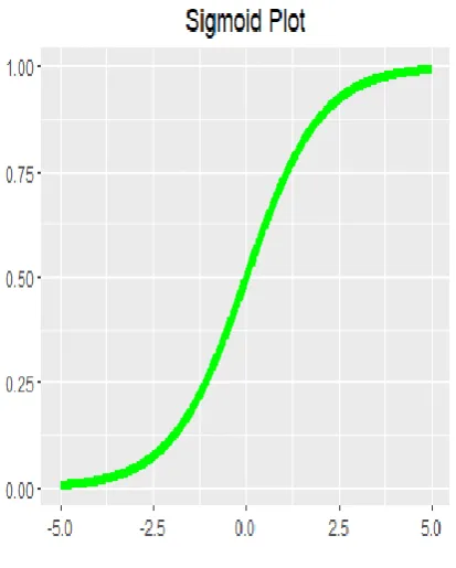
Logistics Regression is a supervised machine learning technique used to solve regression problems having discrete target variable. It takes input as the hypothesis in the sigmoid function such that output is estimated probability. Estimated probability is then converted into either 0 or 1 by taking some threshold. It uses the below equation to find the estimated probability.

Log =β0 + β (variable)

[image:3.595.310.545.66.462.2]

Where p is probability and β’s are coefficients.

Fig. 4 Sigmoid Plot (S-curve)

Without using any sampling techniques and SMOTE logistic regression gives the following results.

Precision: Nan Recall: 0.000 F: Nan AUC: 0.900

After implementing sampling techniques:\

Under Sampling Oversampling Synthetic Data Generation

precision: 0.007 recall: 0.382

F: 0.007 AUC : 0.509

F: 0.030

AUC: 0.906

[image:3.595.64.271.381.639.2]

F: 0.019 AUC: 0.865

Fig.5 ROC Curve1: Best AUC: 0.906

7.2 DECISION TREE

Decision tree is a supervised machine learning algorithm used for both regression and classification problems. Decision tree represents a solution based on certain conditions using graphical representations [3]. First, it chooses the most appropriate variables then splits data using gini index, chi-square, and information gain etc. methods. Decision tree works in two ways, either it grows until the last observation or it splits using some condition. These conditions are max depth, min split, etc. it has a root node, decision node and terminal node.

Without using any techniques decision tree gives the following results.

Precision: 0.706 Recall: 0.176 F: 0.141 AUC: 0.715

(4)

F: 0.035

AUC : 0.917

F: 0.035 AUC:0.872

F: 0.011 AUC: 0.679

Fig.6 ROC Curve2: Best AUC: 0.917

7.3 RANDOM FOREST

Random forest is one of the ensemble technique used in machine learning. It builds the multiple decision trees to get the final result. It can be used for both regression and classification problems. It uses 63.2% of data for each tree to build a model, the remaining data is used to calculate out of the bag error [4]. One of the advantages of using random forest is that it is not sensitive to outliers. That means using this model after under sampling techniques won’t add much value. It will give approximately the same result with under sampling, and this can be verified in below table. Random forest should be implemented if the model is suffering from high variance problem. It works well even without much hyper parameter tuning.

Without using any methods model gives the following results. Precision: 0.921

Recall: 0.515 F: 0.330 AUC: 0.995

After implementing different methods:

F: 0.064 AUC : 0.981

F: 0.368

AUC: 0.996

F: 0.011 AUC:0.935

Fig.7 ROC Curve3:Best AUC: 0.996

8. EVALUATION METRICS

While implementing linear or classification models it's not necessary to separate classes completely by using decision boundaries. It’s 2- dimensional line in case of binary problem and hyperplane in the multiclass problem. An attempt to separate classes completely may lead to overfitting, so instead of getting high accuracy, we should look for a robust model that may misclassify some points. The data points who classified correctly in the positive class is known as true positive and those we don't known as false positive. Similarly, in negative class who predicted correctly is True negative otherwise false negative.

Confusion Matrix

A confusion matrix is a matrix used to evaluate different metrics for classification problem. In case of binary classification problem its 2*2 matrix.

Target

Positive Negative

Model

Positive True Positive False Positive

(5)

To evaluate error measure accuracy is not effective, because the minor class in target outcome having very less contribution. Instead of accuracy other metrics like precision, recall, and f1 score, auc is useful.

Precision

Positive predictive value or precision calculated as below: Precision=

Negative Predictive value

Negative predictive value Calculated as below: Negative Predictive value=

Recall

Recall / Sensitivity calculated as below:

Recall=

Specificity

Specificity calculated as below:

Specificity=

Accuracy

Accuracy calculated as below: Accuracy=

F1 Score

F1 score is harmonic mean of precision and recall and can be find using below formula.

F1=2*

Area under Curve (AUC-ROC)

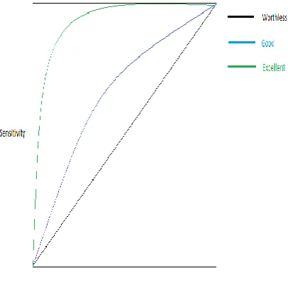
[image:5.595.66.269.543.742.2]

In general, auc gives information about the data points which are not classified correctly. Higher the misclassified data points less auc. The area under curve is a plot having x-axis 1-specificity and y-axis sensitivity. 1-1-specificity is same as false positive Rate and sensitivity are True Positive Rate. In below square plot if curve coincides with diagonal then it’s worthless with AUC 0.50. Middle curve is acceptable but the upper curve gives the excellent result. AUC can be anything between 0.5 to 1.

Fig. 8 ROC Curve, Specificity & Sensitivity

Since after sampling method target outcome have the equal proportion of classes so metrics accuracy can be used. Below table shows only the best result from under sampling, oversampling and synthetic data generation for each models.

Models Precision Recall F1

Score

AUC

Logistic Regression

0.031 0.941 0.030 0.906

Decision Tree

0.036 0.941 0.035 0.917

Random Forest

0.807 0.676 0.368 0.996

9. CONCLUSIONS

It is seen that upon using appropriate sampling techniques, ML models gave better results, except in some cases. Among all models discussed in this paper, Random Forest (RF) has given the best results. That being said, there is not a single sampling technique that gave best results across all the models. After using various sampling techniques with different modelling methods, it is found that using RF in combination with oversampling, gave the best AUC 0.996. Using the above results, days with anomalous behavior are detected. In the further studies, exact time can also be detected after analyzing the variance. The above results can also be used with data generated from other sensors while analyzing & forecasting equipment performance and failures.

10. ACKNOWLEDGMENTS

We would like to express our sincere gratitude to Teras New & Renewable Energies LLP (TNRE LLP) for providing us the opportunity to work on this project. TNRE LLP provides on-premise & cloud based IoT solutions for various manufacturing and energy companies.

11. REFERENCES

[1] Practical Guide to deal with Imbalanced Classification Problems in R. Retrieved from https://www.analyticsvidhya.com/blog/2016/03/practical -guide-deal-imbalanced-classification-problems/ [2] Will, Todd (1999)”Introduction to the Singular Value

Decomposition” Davidson College. www.davidson.edu/academic/math/will/svd/index.html [3] DECISION TREE IN R: STEP BY STEP GUIDE.

Retrieved from

https://www.listendata.com/2015/04/decision-tree-in-r.html

[4] RANDOM FOREST IN R: STEP BY STEP

TUTORIAL Retrieved from

https://www.listendata.com/2014/11/random-forest-with-r.html

[5] I. T. Joliffe, Principal Component Analysis, Springer, New York, NY, USA, 2002.

(6)

[7] Freund, J.E. (1962) Mathematical Statistics Prentice Hall, Englewood Cliffs, NJ. (See pp. 227–228.)

[8] Bryman, A., & Cramer, D. (1994). Quantitative data analysis for social scientists (rev. Taylor & Frances/Routledge.

[9] Bradley, A.P., 1997. The use of the area under the ROC curve in the evaluation of machine learning algorithms. Pattern Recogn. 30 (7), 1145–1159.

[10]Chawla, Nitesh V. (2010) Data Mining for Imbalanced Datasets: An Overview doi:10.1007/978-0-387-09823-4_45 In: Maimon, Oded; Rokach, Lior (Eds) Data Mining and Knowledge Discovery Handbook, Springer ISBN 978-0-387-09823-4 (pages 875–886)

[11] Macskassy, S., Provost, F., 2004. Confidence bands for ROC curves: Methods and an empirical study. In: Proc. First Workshop on ROC Analysis in AI (ROCAI-04). [12] Devinder Kaur, Rajiv Bedi and Dr. Sunil Kumar Gupta,

“Implementation of Enhanced Decision Tree Algorithm on Traffic Accident Analysis”, (IJSRT), ISSN: 2379- 3686, 15th September 2015.