Coverage and Handoff Analysis of 5G Fractal
Small Cell Networks
Jiaqi Chen,
Student Member, IEEE,
Xiaohu Ge,
Senior Member, IEEE,
and Qiang Ni,
Senior Member, IEEE
Abstract—It is anticipated that much higher network capacity will be achieved by the fifth generation (5G) small cell networks incorporated with the millimeter wave (mmWave) technology. However, mmWave signals are more sensitive to blockages than signals in lower frequency bands, which highlights the effect of anisotropic path loss in network coverage. According to the fractal characteristics of cellular coverage, a multi-directional path loss model is proposed for 5G small cell networks, where different directions are subject to different path loss exponents. Furthermore, the coverage probability, association probability, and the handoff probability are derived for 5G fractal small cell networks based on the proposed multi-directional path loss model. Numerical results indicate that the coverage probability with the multi-directional path loss model is less than that with the isotropic path loss model, and the association probability with long link distance, e.g., 150m, increases obviously with the increase of the effect of anisotropic path loss in 5G fractal small cell networks. Moreover, it is observed that the anisotropic propagation environment is having a profound impact on the handoff performance. Meanwhile, we could conclude that the resulting heavy handoff overhead is emerging as a new challenge for 5G fractal small cell networks.
Index Terms—Fractal small cell, anisotropic path loss, coverage probability, handoff.
I. INTRODUCTION
O
NE of the primary goals of the fifth generation (5G) mobile communication is to provide 100Mbps to 1Gbps data rates anytime and anywhere. This goal can be achieved by combining a variety of 5G new technologies, such as massive multi-input multi-output (MIMO), millimeter wave (mmWave), and small cell networks [1], [2]. Base station-s (BSstation-s) equipped with large antenna arraystation-s could achieve directivity gains through precoding/beamforming and could transmit mmWave signals, which results in high data rates. For example, the Samsung’s prototype [3], which is a 4×8 uniform planar array working at 27.925GHz, is able to offer excellent performance, where the reported peak data rate with no mobility is about 1Gbps over a range up to 1.7 kilometers in Line-of-Sight (LoS) transmissions or 200 meters in Non-Line-of-Sight (NLoS) transmissions. The mmWave signals are more sensitive to blockages than signals in lower frequency bands due to the shorter wavelength [4], [5]. Thus, the link distance is reduced when the mmWave signals are transmitted,Jiaqi Chen, Xiaohu Ge (Corresponding author) are with School of Electronic Information and Communications, Huazhong University of Sci-ence and Technology, Wuhan 430074, Hubei, P. R. China e-mail: chen-jq [email protected], [email protected].
Qiang Ni is with InfoLab21, School of Computing and Communications, Lancaster University, Lancaster, LA1 4WA, UK, e-mail:[email protected]. Manuscript received May 02, 2018; revised September 01, 2018, and December 02, 2018; accepted December 04, 2018.
which results in the trend of small cells [6], [7]. In small cell networks, users frequently switch from a small cell BS (SBS) to another SBS since the coverage area of a small cell is significantly smaller than that of a macro cell. The frequent handoff issue in a small cell network with mmWave system be-comes an essential factor that affects the network performance. On the other hand, the fractal coverage of small cells and the propagation environment have the critical influence on the handoff decision. Thus, it is vital to analyze the coverage and handoff performance of 5G small cell networks, considering the anisotropic mmWave signal attenuation in complex urban scenarios.
The coverage performance of small cell networks has been well studied. In small cell networks, multiple classes of BSs such as macro BSs, hotspot BSs, and femtocell BSs are incorporated to provide better coverage for a large number of users. Based on the stochastic geometry theory, the downlink and uplink coverage probabilities were derived for multi-tier heterogeneous cellular networks (HCNs) [8]. In the HCN with a dense small cell topology, the coverage probability for a typical user connecting to the strongest BS signal was analyzed in [9] by incorporating a flexible notion of BS load with a new idea of conditionally thinning the interference field, where penetrating analyses were extended to investigate the impact of network models on the HCN coverage performance. From the point of view of green communication, the coverage probability for a particular cell association scheme, such as the maximum received power association (MRPA) and the nearest base station association (NBA) schemes in the downlink of an HCN, was derived aimed at establishing the fundamental limits on the achievable link and network energy efficiencies [10].
prob-ability and the average rate were obtained. The coverage and rate performance of mmWave cellular networks in major metropolitan cities like Manhattan and Chicago were studied in [13] to confirm that dense BS deployment is the key to achieve both better coverage and higher rate in mmWave cellular networks. Using a distance-dependent LoS probability function calculated by modeling the blockage distribution as a Poisson point process (PPP), a general framework was proposed in [14] to evaluate the coverage and rate performance in mmWave cellular networks. Only two types of transmission links, LoS and NLoS links are considered in the above anal-ysis. In fact, the path loss exponents of different transmission links are entirely different due to the anisotropic propagation environment. In this case, an anisotropic path loss model should be provided to analyze the coverage performance of small cell networks with the mmWave system, compared with the distinction between LoS and NLoS transmission links.
Considering the more irregular coverage of mmWave cel-lular networks and smaller coverage area of a small cell, users have to switch from an SBS to another SBS frequently. An approach for calculating the handoff rate was proposed in [15] based on the angle mobility model. The handoff rate in mmWave 5G systems was investigated in [16], where the typical average handoff interval was shown to be in the range of several seconds. The handoff rate for a user was obtained in [17] for an irregular cellular network with the access point locations modeled as a homogeneous PPP. The vehicular handoff rate and the vehicular overhead ratio were utilized in [18] to evaluate the distance based vehicular mobility performance in 5G cooperative small cell networks. Efficient handoff algorithms were proposed in [19], [20], [21] to minimize the handoff and connection failure rates. In the most handoff analysis literature, the variety of the propagation environment during the user’s moving is ignored in analyzing the handoff performance. However, due to the anisotropic propagation environment, changes in the path loss exponent of the transmission links during the user’s moving have a significant influence on the handoff performance, especially in small cell networks with the mmWave system.
The research efforts in [6–18] were conducted with an assumption that the path loss is isotropic in a cellular scenario, where the most common path loss model is the uniform path loss model,i.e., the path loss exponent is a constant over the entire plane. A piecewise linear path loss model was proposed in [22] where different distance ranges are subject to different path loss exponents. Furthermore, researchers at New York University built a novel channel simulation software named NYUSIM based on the statistical spatial channel model for broadband mmWave wireless communication systems [23], [24]. In [23], the path loss exponents of LoS and NLoS transmissions were configured as different constants. However, our work in [25] indicated that the measured wireless cellular coverage boundary is irregular with respect to directions, and the statistical fractal characteristic of coverage boundary was proved to exist widely. Such a fractal characteristic is illustrated by the spectral density power-law behavior and the slowly decaying variances in the angle domain [25]. More-over, in [26] the single cell coverage boundary was proved
to bear a visible burst pattern, and the probability density function (PDF) of the single cell boundary was shown to have the heavy tail characteristic. In [27], the fractal coverage characteristic was first used to evaluate the performance of small cell networks. From the above result, it is evident that the propagation environment is anisotropic in a mmWave scenario. Although there exist a large amount of meaningful and essential studies for performance analysis of the small cell networks with mmWave, the impact of such anisotropic propagation environments is still not well investigated. Along with the prosperity of machine learning, rich learning schemes [28] obviously facilitate the research of the complex and accurate anisotropic path loss models.
In this paper, based on the fractal characteristics of cellular coverage [25], a multi-directional path loss model is proposed for 5G fractal small cell networks, where different directions are subject to different path loss exponents. Based on the proposed multi-directional path loss model, the coverage per-formance in SINR and rate terms are analyzed to estimate the impact of the anisotropic propagation environment. The handoff decision is made based on the association scheme and the channel state. Some existing analysis for the handoff performance works based on the assumption that the nearest neighbor SBS is the one with the highest SINR. However, the association state with the maximum SINR scheme is more complex in the anisotropic scenario than in the isotropic scenario. The association probability with the multi-directional path loss model is investigated to imply the influence of the anisotropic propagation environment and to lay the foundation for handoff analysis. Furthermore, the handoff performance of 5G fractal small cell networks is evaluated by the handoff probability and handoff rate. The handoff probability implies the performance of an individual handoff operation, and the handoff rate illustrates the overall network performance. The main contributions of this paper are as follows:
1) Based on the fractal characteristics of cellular cover-age, a multi-directional path loss model is proposed to analyze the impact of an anisotropic propagation environment on the performance of 5G fractal small cell networks, where different directions are subject to different path loss exponents.
The rest of the paper is organized as follows. Section II describes the system model. The coverage and association probability analyses are presented in Section III. The handoff probability and handoff rate are derived in Section IV. The simulation results are presented in Section V. Finally, conclu-sions are drawn in Section VI.
II. SYSTEMMODEL
We consider a downlink small cell network in this paper. Without loss of generality, SBSs are assumed to be deployed randomly over an infinite plane R2 and modeled as a
homo-geneous PPP of intensityλ[29]:
Φ ={xi, i= 1,2,3, . . .}, (1)
wherexi is a Polar coordinate denoting the location of SBSi, i.e., xi = (ri, θi), with radial coordinate ri denoting the distance between SBSi and the coordinate origin, and angular coordinate θi. A typical user is assumed to be located at the coordinate origin, denoted as u0.
Considering that the mmWave technology is excepted to be adopted in 5G small cell networks, a multi-directional path loss model is proposed in this section and aims at analyzing the impact of anisotropic propagation environment on the performance of mmWave small cell networks. What’s more, the channel model is introduced.
A. Multi-directional Path Loss Model
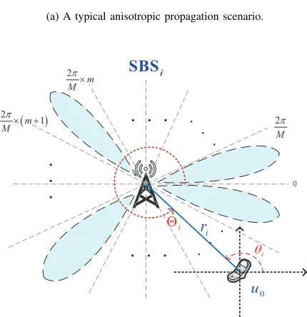
With the emerging mmWave technology, researchers have examined the mmWave technology in some typical environ-ments, e.g., an urban scenario with LoS transmissions, an urban scenario with NLoS transmissions, and the near-ground propagation in the forest. The empirical path loss exponents for the above three scenarios were reported as 2.1 [30], 3.19 [30], and 4 [31], respectively. It can be found that the path loss exponents are entirely different in these scenarios. Considering that the three typical propagation environments are irregularly distributed around SBSs, the links from a user to SBSs possibly pass through different environments such that the path loss exponents of these links are different. In this case, a uniform path loss model cannot be used to investigate the real anisotropic radio propagation. Thus, a multi-directional path loss model is proposed in this paper to evaluate the radio propagation in an anisotropic path loss scenario. A typical anisotropic path loss scenario is shown in Fig. 1a, where a user moves from point A to point D along the red line. The link between the user and a particular SBS passes through the wood when the user is in the range between A and B. The link between the user and the SBS passes through buildings when the user is in the range between B and C. These links are NLoS. The link between the user and the SBS is LoS when the user is in the range between C and D.
In this model, the coverage area centered at an SBS is equal-ly partitioned intoM sections, and the path loss exponents of
M sections are assumed to be different, where the value ofM
is artificially configured to model the anisotropic characteristic of a given propagation environment. WhenM is large enough, the values of the path loss exponents in M sections could
A
B
D
SBS
User
C
(a) A typical anisotropic propagation scenario.
2
M p ( )
2 1
m M
p
´ +
2
m M
p ´
i
Q
SBS
i0
u
i
r
i q
[image:3.612.329.544.247.469.2](b) The multi-directional path loss model.
Fig. 1. The typical anisotropic path loss scenario and model.
be regarded as the samples of the path loss exponent around the SBS. The sequence Ωi = {αim} denotes a stochastic process of the path loss exponent of SBSi, composed of the random variables αim with the index m(m= 1,2, . . . , M). The anisotropic characteristic of the propagation environment could be analyzed with statistical methods based on theseM
samples. Considering that the value ofM needs to be given to characterize the system performance, we show in Section V by simulation that the impact of M on the performance becomes stable when the value of M is larger than 400.
on, are independent [32], [33]. Considering that the sections in different directions are non-overlapping, the obstacles in different sections are independent. Therefore, in this paper the path loss exponent of the m-th section of SBSi(i= 1,2, ...), denoted as αim, is assumed to be independently identically distributed (i.i.d.) random variables uniformly distributed with mean µand variance σ, and its PDF is given as
f(αim) =
1
2√3σ, αim∈
[
µ−√3σ, µ+√3σ
]
. (2)
Note that the path loss exponent of them-th section at SBSiis independent of the m-th section at SBSj(j̸=i),i.e., αim̸= αjm.
A possible solution to obtain the path loss exponents of
M sections of an SBS in practice is introduced as follows. In order to let the SBS perceive the existence of the mobile phone at any time, the mobile phone must report the channel state information (CSI) back to the SBS regularly, or must immediately return when the SBS asks [34]. If the SBS is allowed to obtain the mobile phone’s location, the path loss exponent can be estimated by a least square’s method at the SBS based on the CSI and the location reported by the mobile phone. Considering the urban scenario, every SBS serves many users around it. The SBS collects the CSI and the locations of all online mobile phones, and then computes the path loss exponent of each section using the collected data from the section.
According to the 3GPP path loss models summarized in TR 38.900 [30], the path loss exponent in UMi-Street Canyon scenario is 2.1 when the link distance is smaller than the breakpoint distance, and that becomes 4 when the link dis-tance is larger than the breakpoint disdis-tance. The characteristic mutations of path loss exponent occur at the breakpoint. Considering a mmWave system in the small cell network that
fc = 24GHz, the height of SBS is 5m, the height of user is 1.5m, the breakpoint distance is calculated as 640m, which comfortably exceeds the average coverage radius of an SBS given as √1
πλ ≈56m. We consider the 5G fractal small cell networks with high density in which the link distances are usually smaller than the breakpoint distance. In this case, the difference in path loss exponents of different directions is mainly considered in this paper. The multi-directional path loss over the link between SBSi and the typical useru0 is set
as
L(xi) =r−i αim, (3)
when 2Mπ(m−1) ≤Θi < 2Mπm (m= 1, . . . , M), where Θi
is the angle of the vector from SBSitou0, which is calculated
to locate the section that the user stays in, shown in Fig. 1b. The angle Θi is given as
Θi=
{
θi+π θi∈[0, π)
θi−π θi∈[π,2π)
. (4)
Such a multi-directional path loss model can be degraded into the isotropic path loss model with the uniform path loss exponent over the entire plane when σ = 0, i.e.,
αi1 = αi2 = · · · = αiM = αc = µ as a constant with
SBS
[image:4.612.334.547.64.251.2]Cell boundary with the multi-directional path loss model Cell boundary with the isotropic path loss model
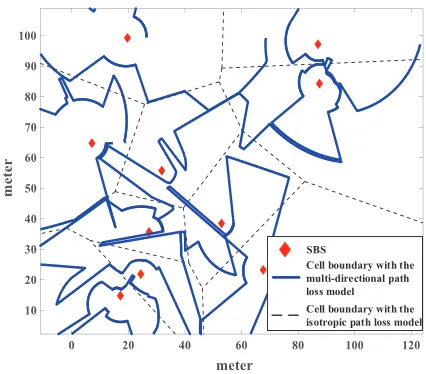
Fig. 2. Illustration of 5G fractal small cell network structure with the multi-directional path loss model (M = 5,µ = 4,σ = 1), compared with the isotropic path loss model.
probability 1. The isotropic path loss model could be expressed as L1(x
i) =r−i µ.
To illustrate the 5G fractal small cell network structure, assume that a user is associated with the SBS from which the user receives the maximum SINR, and users only suffer the path loss during propagation. Every cell is assumed to include only one SBS. The locations at which the user receive equal SINRs from the two adjacent SBSs, make up the cell boundaries. For the multi-directional path loss model, the blue solid lines in Fig. 2 depict cell boundaries inside which a polygon corresponds a cell coverage. For the traditional isotropic path loss model, the SBS with the maximum SINR is the closest SBS for the user. In this case, the cell boundary can be obtained through the Delaunay Triangulation method [35] expressed as the black dashed lines in Fig. 2.
What is more, the carrier frequency factor fc in the path loss,P L= 32.4 + 20 lg (r) + 20 lg (fc) (dB)[30], is normal-ized to simplify the analysis of the impact of the anisotropic path loss, considering that the same carrier frequency is used at all SBSs.
B. Channel Model
When the channel fading of each transmission link is assumed to be governed by the i.i.d. Rayleigh fading, the received signal power atu0 from SBSi is given as
Pi=PTGihiL(xi), (5)
where hi denotes the power gain from Rayleigh fading be-tween u0 and SBSi, which is assumed to be governed by an exponential distribution with mean 1 similar to [11]. For simplicity, but without loss of generality, all SBSs are assumed to transmit with the same transmission powerPT.Gi denotes the antenna gain obtained from the SBSi andu0.
TABLE I
THE PROBABILITY DISTRIBUTION OF ANTENNA GAINGi
Value g1=MtMr g2=Mtmr g3=mtMr g4=mtmr
Probability p1=ϕ2πtϕ2πr p2=ϕ2πt (
1−ϕr
2π
) p3=
(
1−ϕt
2π
)
ϕr
2π p4=
(
1−ϕt
2π
) (
1−ϕr
2π
)
its serving SBS will estimate the channels including angles of arrivals and fading gains, and then adjust their antenna steering orientations accordingly to exploit the maximum antenna gain. Errors in channel estimation are neglected, and so are errors in time and carrier frequency synchronization in this paper. Thus,MtandMrare the main lobe gains of the SBS and user, respectively;mtandmrare the side lobe gains of the SBS and user, respectively; ϕtandϕr denote the main lobe width and side lobe width of the SBS and user, respectively. The antenna gain of the desired link is MtMr, and the antenna gain of the interfering link is a random variable with the distribution shown in Table I [14].
In order to obtain the best channel condition, a user is configured to be associated with a particular SBS based on the SINR value,i.e., when the SINR value of the link between the user and this SBS is the maximum. The SBS associated with the typical user u0is denoted as SBSk, where
k= argmax xi∈Φ
SINR (xi), (6)
with
SINR (xi) = Pi I(xi) +σn2
= PTMtMrhir −αi
i
∑
xj∈Φ,j̸=i
PTGjhjr− αj
j +σ2n
, (7)
which is the SINR value of the link betweenu0and SBSiwith σn2denoting the noise power andI(xi)denoting the aggregate interference. The path loss exponentsαi andαj in (7) depend on the angles Θi andΘj of the vectors from SBSi and SBSj to the typical user, respectively.
III. COVERAGE ANDASSOCIATIONPROBABILITY
In this section, the coverage and association probabilities of 5G fractal small cell networks are derived based on the multi-directional path loss model. Numerical analyses of the coverage and association probabilities are conducted to evalu-ate the performance impacted by the anisotropic propagation environment.
A. Coverage Probability
We analyze the coverage performance with the multi-directional path loss model of 5G fractal small cell networks in SINR and rate terms. The expressions for the SINR and rate coverage probability with the multi-directional path loss model are derived. The SINR coverage probability to the point of view of the typical user u0 is the probability that the desired received SINR at u0 is larger than a threshold
τ. Considering the maximum SINR association, the SINR coverage probability is given as
PC(τ) =Pr
{ max xi∈Φ
SINR (xi)> τ
}
. (8)
Lemma 1. Based on the Lemma 1 in [36], when the SINR
threshold τ > MtMr
mtmr, at most one SINR can be greater than
τ.
Proof:See Appendix A.
Theorem 1. The SINR coverage probability for the typical
user at the origin is given as
PC(τ) =
λπ √
3σ
∫ ∞
0
∫ µ+√3σ
µ−√3σ
rexp
(
−√λπ2 3σ
4
∑
l=1 pl
×
∫ µ+√3σ
µ−√3σ
(
τ rαigl
MtMr
)2
α
α csc
( 2π
α
)
dα− τ r
αiσ2
n
PTMtMr
dαidr. (9)
Proof:See Appendix B.
Furthermore, we analyze the distribution of the achievable rate R0 of 5G fractal small cell networks with the multi-directional path loss model. The achievable rate is defined as
R0=BWlog2
(
1 + max xi∈Φ
SINR (xi)
)
, (10)
where BW is the bandwidth assigned to the typical user u0. The rate coverage probability is the probability that the
achievable rate of the typical user is larger than the threshold
γ, which is expressed as
PR(γ) = Pr{R0> γ}
= Pr {
BWlog2
(
1 + max xi∈Φ
SINR (xi)
)
> γ
}
= Pr {
max xi∈Φ
SINR (xi)>2
γ BW −1
}
=PC
( 2
γ BW −1
)
. (11)
To express the impact of the multi-directional path loss model on the coverage performance of the 5G fractal small cell network, numerical results of the SINR and rate coverage probabilities are presented considering the factors including the SINR thresholdτ, the rate thresholdγ, the SBS densityλ, and the meanµand the varianceσof the path loss exponent. The default parameters are set as: PT = 30dBm, BW = 500MHz,σ2n=−174dBm/MHz×500MHz=−87dBm [37],
10 20 30 40 50 60
SINR threshold (dB)
0 0.1 0.2 0.3 0.4 0.5 0.6 0.7 0.8 0.9 1
SINR coverage probability
Analysis of Isotropic path loss Simulation for Isotropic path loss Analysis of =0.4
[image:6.612.318.553.54.246.2]Simulation for =0.4 Analysis of =0.8 Simulation for =0.8 Analysis of =1 Simulation for =1
Fig. 3. The SINR coverage probability with respect to the SINR threshold τ, considering different variances of the path loss exponent.
Fig. 3 illustrates the SINR coverage probability with respect to the SINR threshold τ, considering different variances σ
of the path loss exponent. The SINR coverage probability decreases with the increase of the SINR threshold. When the variance is equal to zero, i.e.,σ= 0, the path loss exponent is a constant with probability 1, and is equal to the mean
µ. Thus, the case with σ = 0 represents the isotropic path loss model in this paper. When the SINR threshold is fixed, the SINR coverage probability decreases with the increase of the variance σ, which indicates that the anisotropic path loss model has a negative influence on the coverage performance of the small cell network. According to the proof of Lemma 1, the result shows numerically that this SINR coverage probability model holds very accurately.
Fig. 4 shows the SINR coverage probability with respect to the variance of the path loss exponent σ, considering different mean values µ. The larger mean value µ results in that the SINR coverage probability increases, which implies that the coverage performance is better in the higher path loss attenuation environment due to the more severe attenuation of the interference signal. When the mean µ is fixed, the SINR coverage probability decreases with the increase of the variance σ, which shows that the coverage performance is better in the more stable propagation environment, especially in the isotropic propagation environment with the caseσ= 0. It is because the path loss exponents of a part of interference links are so small in the anisotropic propagation environment that increase the aggregate interference power compared to the isotropic path loss model.
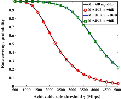
Fig. 5 illustrates the rate coverage probability with respect to the achievable rate thresholdγ, considering different antenna gains. The rate coverage probability increases with the larger ratio of the main lobe gain to the side lobe gain Mt
mt. It can be found in the figure that the red and black lines with Mt
mt = 10dB−0dB = 5dB−(−5)dB = 10dB ate below the green and blue lines with Mt
mt = 20dB−0dB = 10dB−(−10)dB = 20dB. What’s more, the rate coverage
0 0.2 0.4 0.6 0.8 1
Variance of path loss exponent
0.1 0.2 0.3 0.4 0.5 0.6 0.7
SINR coverage probability
Analysis of =4 Simulation for =4 Analysis of =5 Simulation for =5 Analysis of =6 Simulation for =6
Fig. 4. The SINR coverage probability with respect to the variance of the path loss exponentσ, considering different mean valuesµ.
500 1000 1500 2000 2500 3000 3500 4000 4500 5000
Achievable rate threshold (Mbps)
0 0.1 0.2 0.3 0.4 0.5 0.6 0.7 0.8 0.9 1
Rate coverage probability
Mt=5dB mt=-5dB Mt=10dB mt=0dB Mt=10dB mt=-10dB Mt=20dB mt=0dB
Fig. 5. The rate coverage probability with respect to the achievable rate thresholdγ, considering different antenna gains.
probability is independent from the values of and when the ratio of the main lobe gain to the side lobe gain Mt
mt is fixed.
B. Association Probability
[image:6.612.61.296.57.245.2] [image:6.612.319.553.292.482.2]In this paper, a user is assumed to be associated with the SBS that leads to the maximum received SINR. The association probability with respect to the distancerbetween
u0 and the desired SBS SBSr is expressed as
PA(r) = Pr
{
SINR (r) = max xi∈Φ
SINR (xi)
}
, (12)
SINR (r) =PTMtMrhrr −αr
I(r) +σ2 n
, (13)
where hr, and αr denote the antenna gain, power gain from Rayleigh fading, and path loss exponent of the link betweenu0
and the desired SBS SBSr, respectively.I(r)is the received interference of the useru0.
Considering the difficulty of calculating the association probability due to the complex expression of SINR, an ap-proximation that greatly simplifies the analysis is that the user is associated with the SBS that leads to the maximum received power. The following Lemma shows that the approximation has the high accuracy, and the accuracy increases with the narrower main lobes at the transmitter and receiver.
Lemma 2. The probability that SINR (xk) is the maximum
is at least (
1− ϕt
360
) ( 1− ϕr
360
)
when the corresponding re-ceived signal powerPk is maximum.
Proof: See Appendix C.
Note that the system level simulations are given for the probability in Lemma 2, expressed as Pr{SINR (r)|P(r)}. The results are shown in Table II and imply that the probability is higher when the narrower main lobes are equipped at the transmitter and receiver. In this case, the probability that SINR (r) is the maximum can be approximated by the probability that P(r) is the maximum. Based on Lemma 2, the association probability is further expressed as
PA(r)≈Pr
{
P(r) = max xi∈Φ
Pi
}
, (14)
where P(r) denotes the received signal power at u0 from SBSr, expressed asP(r) =Grhrr−αr.
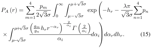
Theorem 2. The association probability with respect to the
distance r betweenu0 and the desired SBS SBSr is approxi-mately given as
PA(r) =
4
∑
m=1
pm
2√3σ
∫ ∞
0
∫ µ+√3σ
µ−√3σ exp
(
−hr− λπ √
3σ 4
∑
n=1 pn
×
∫ µ+√3σ
µ−√3σ
(
gm
gnhrr −αr
)−2
αi
Γ
(
2 αi
)
αi
dαi
dαrdhr. (15)
[image:7.612.49.301.581.662.2]Proof: See Appendix D.
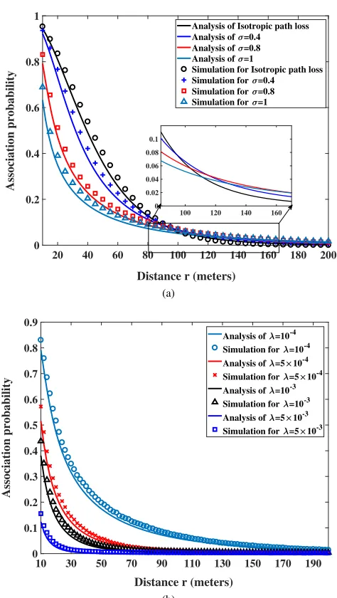
Fig. 6a shows the association probability with respect to the distancerbetweenu0and the desired SBS SBSr, considering different variances σ. When the variance of the path loss exponent is fixed, the association probability decreases with the increase of the distance r between u0 and the desired SBS SBSr. When the distance r is smaller than 80 meters,
the association probability increases with the decrease of the variance σ. When the distance r is larger than 160 meters, the association probability increases with the increase of the varianceσ. The realistic association of users in small cell net-works is more complicated than the NBA scheme. The result also implies that the nearest base station association scheme is not the desired method to obtain the best channel gain in small cell networks with mmWave. Thus, we need to pay more attention to the novel association scheme when analyzing the performance of small cell networks with mmWave. Fig. 6b shows the association probability with respect to the distance
rbetweenu0and the desired SBS SBSr, considering different intensities of SBSsλ. The variance of the path loss exponent is set asσ= 0.8. When the distanceris fixed, the association probability decreases with the increase of the intensity of SBSs. What’s more, we now focus on the approximation in Lemma 2 by comparing the theoretical and simulated results for association probability in Fig. 6. As expected, the simulated and analytical results match reasonably well.
Fig. 7 shows the association probability with respect to the variancesσ, considering different distancesrbetweenu0 and SBSr. The mean value of the path loss exponent in this figure is equal to 5 to ensure that the minimum value of the path loss exponent is larger than 2. When the distancerbetweenu0
and the desired SBS SBSris shorter than 90m, the association probability decreased with the increase of the varianceσof the path loss exponent. When the distance is larger than 110m, the association probability has a peak value at particular variances.
IV. HANDOFFPERFORMANCE
In particular, the handoff is crucial for keeping users con-nected while moving around. Frequent handoff in small cell networks affects not only service quality of users but also network performance, such as throughput and energy effi-ciency. Conditional handoff analysis is based on the isotropic propagation environment. However, the negative influence of the anisotropic environment on the handoff performance is predictable in future small cell networks. In this section, the handoff probability and handoff rate are derived based on the user random walk mobility model to investigate the impact of the multi-directional path loss model.
A. Handoff Probability
Assumed that the serving SBS of the typical useru0 at the
locationl0 is denoted as SBSr,i.e., the SINR of SBSrat the
locationl0is the maximum. Letl0 andl1respectively denote the locations at the start and end of a short time movement, and the moving time is the time interval between the end of the last handoff decision and the begin of the next one. 3GPP Standard defines six handoff events for cellular networks [40]. In this paper, the analysis of handoff performance with the multi-directional path loss model focuses on the most common Event A2. The Event A2 occurs when the SINR of the serving SBS becomes smaller than a thresholdτh, and the trigger condition can be expressed as
TABLE II
THE PROBABILITY THATSINR (r)IS THE MAXIMUM WHENP(r)IS THE MAXIMUM(r= 50m).
ϕt 7◦ 20◦ 60◦ 60◦ 20◦ 7◦
ϕr 60◦ 60◦ 60◦ 20◦ 10◦ 10◦
Pr{SINR (r)|P(r)} 0.9176 0.9035 0.8822 0.9036 0.9553 0.9709
20 40 60 80 100 120 140 160 180 200
Distance r (meters)
0 0.2 0.4 0.6 0.8 1
Association probability
Analysis of Isotropic path loss Analysis of =0.4
Analysis of =0.8 Analysis of =1
Simulation for Isotropic path loss Simulation for =0.4
Simulation for =0.8 Simulation for =1
100 120 140 160 0
0.02 0.04 0.06 0.08 0.1
(a)
10 30 50 70 90 110 130 150 170 190
Distance r (meters)
0 0.1 0.2 0.3 0.4 0.5 0.6 0.7 0.8 0.9
Association probability
Analysis of =10-4 Simulation for =10-4 Analysis of =5 10-4 Simulation for =5 10-4 Analysis of =10-3 Simulation for =10-3 Analysis of =5 10-3 Simulation for =5 10-3
[image:8.612.56.293.133.553.2](b)
Fig. 6. The association probability with respect to the distancerbetweenu0 and the desired SBS SBSr, considering different variances of the path loss
exponent and the intensities of SBSs.
where τhys is a hysteresis parameter added for reducing re-dundant handoffs (e.g. ping-pong effect), andr˜is the distance between the serving SBS and the user at the new location
l1. Once inequality (16) is satisfied for the user, an Event A2 handoff is triggered, and the user needs to select a suitable tar-get SBS. In this case, the handoff probability,PH(vt), denotes the probability that a handoff occurs when the user moves a distancevt, which is expressed asPH(vt) =
∫∞
0 Pr{A2}dr.
When the distance between the serving SBS and the user at location l0 is r, the probability that the Event A2 occurs is
0 0.5 1 1.5
0 0.1 0.2 0.3 0.4
Analysis of r=50m Analysis of r=70m Analysis of r=90m Simulation for r=50m Simulation for r=70m Simulation for r=90m
0 0.5 1 1.5
Variance of the path loss exponent
0 0.02 0.04 0.06
Association probability
[image:8.612.319.544.149.331.2]Analysis of r=110m Analysis of r=130m Analysis of r=150m Simulation for r=110m Simulation for r=130m Simulation for r=150m
Fig. 7. The association probability with respect to the variancesσ, considering different distancesrbetweenu0and SBSr.
given as
Pr{A2}= Pr{SINR (˜r)< τh−τhys}. (17)
Before calculating the handoff probability, the relationship between the locationsl0andl1are considered. The movement
of a user is assumed to be governed by a random walk mobility model in this paper. The user moves from its original location to a new location by randomly choosing a directionφ and a speedv, where the speed and direction are both chosen from pre-defined ranges[vmin, vmax]and[0,2π), respectively. Such a random walk mobility model is shown in Fig. 8a, whereu0
moves from the locationl0 tol1,Θi is the angle between the horizontal line and the line crossing throughl0 and SBSi,Θ˜i is the angle between the horizontal line and the line crossing throughl1and SBSi,riandr˜iare the distances between SBSi and l0,l1, respectively, t is the user moving time, and vt is
the distance of the user moving with the speedv and timet. The relationship between the locations l0 andl1 is expressed
as
˜
r2i =r2i + (vt)2+ 2vtricos (φ−Θi), (18)
˜
Θi= Θi+ arctan
(
vtsin (φ−Θi) r+vtcos (φ−Θi)
)
. (19)
Two special cases are considered in the derivation. One case is that the user moves away from the serving SBS: SBSr,i.e.,
SBSi 0 l 1 l i r i ri ri vt j i Qi Q Q i Q
(a) The random walk mobility model.
2 p
r
vt
m-th section 2 r m M p - Q(b) The scenario that user moves at the directionφ= Θr+π
[image:9.612.316.561.92.274.2]2.
Fig. 8. The random walk mobility model with the multi-directional path loss model.
Case 1: φ = Θr. In this case, the path loss exponent of the link between the user and the serving SBS is unchanged. When the user moves a distance vt, the received SINR of the serving SBS at the user is given as
SINR0(˜r) = PTMtMr ˜
hr(r+vt)− αr
I(r+vt) +σ2
n
, (20)
whereh˜r is the power gain from Rayleigh fading at the new location, which is independent ofhr.
The handoff probability is expressed as
PH0 (vt) = ∫
r
Eαr [
Pr{SINR0(˜r)< τh−τhys|αr
}
PA(r|αr)
]
dr,
(21) with the conditional association probability following (15)
PA(r|αr) = 4 ∑ m=1 pm ∫ ∞ 0 exp (
−hr− λπ √ 3σ 4 ∑ n=1 pn ×
∫ µ+√3σ
µ−√3σ
(
gm
gnhrr −αr
)−2
αi Γ ( 2 αi ) αi dαi
dhr. (22)
Theorem 3. When the user moves to the direction φ= Θr,
the handoff probability is
PH0 (vt)
=
∫ ∞
0
∫ µ+√3σ
µ−√3σ
( 1−exp
(
−
(
τh−τhys
PTMtMr
)
σ2n(r+vt)αr )
×exp
−√λπ2
3σ 4 ∑ l=1 pl ∫ α (
(τh−τhys)(r+vt)αrgl
MtMr
)2
α
csc(2απ)
α dα × (4 ∑ m=1 pm ∫ ∞ 0 exp (
−hr− λπ √ 3σ 4 ∑ n=1 pn ×
∫ µ+√3σ
µ−√3σ
(
gm
gnhrr −αr
)− 2
αi Γ ( 2 αi ) αi dαi
dhr
dαrdr.
(23)
Proof:See Appendix E. Case 2: φ= Θr+π
2. As shown in Fig. 8b, the path loss
exponent is unchanged when the moving distance satisfies
vt≤rtan(2Mπm−Θr). When the moving distance is larger thanrtan(2Mπm−Θr), the path loss exponent changes. Then, the received SINR of the serving SBS at the user is given as
SINR90(˜r) =
PTMtMr˜hr
(
r2+ (vt)2)−
˜ αr
2
I
(√
r2+ (vt)2
) +σ2
n
, (24)
where α˜r denotes the new path loss exponent of the link between the serving SBS and the user located at sections except for them-th section. Given that the distancerbetween the user and the serving SBS is fixed and known, angleΘr is assumed to be uniformly distributed in[0,2π)and independent of the distance r [41]. In this case, ∆Θ = 2Mπm−Θr is uniformly distributed in [0,2Mπ). The handoff probability is expressed as
PH90(vt)
=M 2π ∫ 2π M 0 (∫ vt tan(∆Θ) 0
Pr{SINR90(˜r)< τh−τhys }
PA(r)dr
+
∫ ∞
vt tan(∆Θ)
Eαr [
Pr{SINR90(˜r)< τh−τhys|α˜r=αr
}
×PA(r|αr)]dr)d∆Θ. (25)
The detailed calculation is similar to the Theorem 3, which is omitted here. The final expression of the handoff probability withφ= Θr+π
2 is not shown here.
B. Handoff Rate
and the SBSs. Hence, the overall handoff overhead is directly proportional to the handoff rates.
To easily evaluate the handoff overhead, the handoff rate is defined as the average number of handoffs per unit time. According to the handoff control protocols [42], the handoff decision procedures are periodically executed, where the signal detection and information exchanging between the user and the original associated SBS are conducted in each given period. Such a period is denoted as the detection interval td. Thus, in this paper Monte-Carlo simulations are utilized to analyze the handoff rate of 5G fractal small cell networks, with the multi-directional path loss model.
We consider a small cell network deployed in an urban area, and the network consists of a user and a varying number of SBSs. The user is initially located at the central of a circular area with radius equal to 1000m, and SBSs are randomly distributed in the area. Some parameters related to system model are the same as those in Section III. The user moves to a random direction at a speedv. In each periodtd, the channel state information is reported to the serving SBS by the user, and a handoff decision mechanism is executed. We assume that a perfect initial cell search can be performed, and thus the user can discover SBSs correctly when a handoff occurs. The number of handoffs in 1000 seconds is recorded to calculate the handoff rate.
V. SIMULATION RESULTS
The handoff probability and handoff rate are analyzed for 5G fractal small cell networks with the multi-directional path loss model (where the uniform path loss model is treated as a special case with σ = 0) in this section. The default parameters are configured as in Section III. The SINR thresh-old for handoff with a hysteresis parameter is configured as
τh−τhys= 0dB.
Fig. 9 shows the handoff probability with respect to the moving distance vt in the two special cases, considering different variances of the path loss exponent. In this figure, the number of sections of each SBS is configured asM = 3. The handoff probability increases with the increase of the moving distance in a detection interval. And the handoff probability increases with the increase of the variance of the path loss exponent. The difference between the handoff probabilities in the case 1 and case 2 could be ignored at the same condition with moving distance and variance of the path loss exponent. The results imply that the direction of the user movement has no influence on the handoff performance.
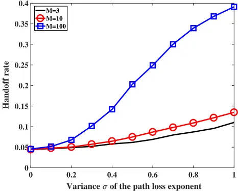
Fig. 10 illustrates the handoff rate with respect to the variance σ of the path loss exponent, considering different values ofM. For the analysis of the handoff rate, the detection interval td is configured as 1 second, and the user moving speed v is 5m/s. The handoff rate increases with increase of the variance σ when the value of M is fixed. The slope of the curve with M = 100, is much larger than slopes of the other curves, i.e., the handoff rate with larger M is growing more than the handoff rate with small M. The result shows that the complex anisotropic propagation environment has negative impact on the handoff performance, and the handoff
0 5 10
0.05 0.1 0.15
Handoff probability
Case 1: = r
Isotropic path loss =0.4
=0.8 =1
0 5 10
Moving distance vt
0.05 0.1 0.15
[image:10.612.319.539.60.247.2]Case 2: = r+ /2
Fig. 9. The handoff probability with respect to the moving distancevtin the two special cases, considering different variances of the path loss exponent.
0 0.2 0.4 0.6 0.8 1
Variance of the path loss exponent
0 0.05 0.1 0.15 0.2 0.25 0.3 0.35 0.4
Handoff rate
M=3 M=10 M=100
Fig. 10. The handoff rate with respect to the varianceσ of the path loss exponent, considering different values ofM.
probability analyzed based on the isotropic path loss model and the actual handoff probability have a huge difference in more complex anisotropic propagation environment.
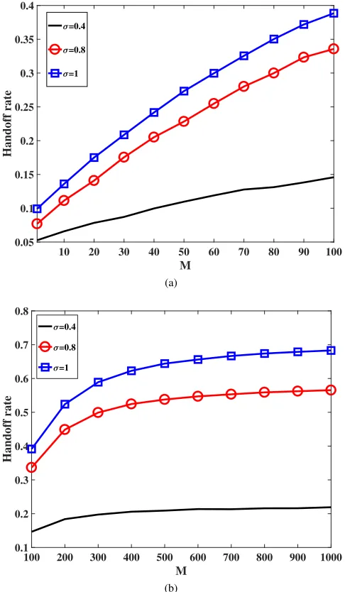
Fig. 11 shows the handoff rate with respect to M, con-sidering different variancesσ of the path loss exponent. The handoff rate increases with the increase of M, the number of sections of each SBS. In Fig. 11a, the value of M is in the range of [10,100], and the handoff rate increases rapidly with the increase ofM. In Fig. 11b, the value of M is in the range of[100,1000], the increase of the handoff rate becomes slowdown whenMis larger than 400. The impact ofM on the handoff rate becomes stable whenM is larger than 400 which advises that the coverage region of an SBS can be equally partitioned into 400 sections in practice.
[image:10.612.322.555.293.480.2]10 20 30 40 50 60 70 80 90 100
M
0.05 0.1 0.15 0.2 0.25 0.3 0.35 0.4
Handoff rate
=0.4
=0.8
=1
(a)
100 200 300 400 500 600 700 800 900 1000
M
0.1 0.2 0.3 0.4 0.5 0.6 0.7 0.8
Handoff rate
=0.4
=0.8
=1
[image:11.612.54.297.57.474.2](b)
Fig. 11. The handoff rate with respect toM, considering different variances σof the path loss exponent.
l1 is zero due to 2Mπ approaching zero when M approaches
infinity. In this case, the path loss exponent of the link at each detection time is an independent random variable. The limit of the handoff rate of 5G fractal small cell networks is influenced by the distribution of the path loss exponent, not influenced by the value of M. And the increase percentage of the handoff rate with the large variance over that with low variance is more than 100% when the large variance is twice as much as the low variance.
VI. CONCLUSIONS
The small cell network is a promising technology for 5G mobile communication systems to increase the network capac-ity. Considering the complex environment in urban scenarios, the anisotropic path loss effect cannot be ignored any more. A multi-directional path loss model was proposed to analyze the impact of the anisotropic path loss exponent on performance in 5G fractal small cell networks. The new coverage probability, association probability and handoff probability were derived
based on the proposed multi-directional path loss model. Numerical results indicate that the association probability with short link distance, e.g., 50m, decreases obviously with the increase of the effect of anisotropic path loss in 5G fractal small cell networks. Moreover, it was observed that the handoff probability with the multi-directional path loss model is larger than the handoff probability with the isotropic path loss model. When the coverage area of each SBS is equally partitioned into 400 sections, the handoff performance can be stably analyzed with the multi-directional path loss model. When the multi-directional path loss model with specific parameters for a special scenario is obtained, the association and handoff probability can be calculated directly based on the statistic characteristic of the measured parameters, which can provide straightforward guidance for the deployment of wireless communication networks.
APPENDIXA PROOF OFLEMMA1
Proof: Let SINR (xi) be denoted as bi, and ai represent PTGihir−i αi. We have
bi=
MtMrai
Gi ∑
j̸=i aj+σ2n
=
MtMrai
Gi ∑
Φ
aj+σn2−ai
=⇒ ∑ ai
Φ
aj+σ2n
= 1
1 + MtMr
Gibi
=⇒∑
Φ
1 1 + MtMr
Gibi
+ σ
2 n
∑
Φ
aj+σn2
= 1. (26)
Then following the proof of Lemma 1 in [36], (26) could be satisfied if only one of the bi (i∈R+) is greater than
MtMr
mtmr, i.e.,
MtMr
Gibi <1, and
1 1+MtMr
Gibi
> 1
2, because the value
of Gi is always greater or equal to mtmr. Assumed that two bi are greater than MmtMr
tmr, denoting asb1, b2. Therefore,
1 1+MtMrG
1b1
> 1 2,
1 1+MtMrG
2b2
> 1 2, and
1 1+MtMrG
1b1
+ 1
1+MtMrG
2b2
> 1
which is in contradiction with (26). This contradictory situa-tion occurs when morebiare greater than MmtMr
tmr. In this case, at most one bi can be greater than MmtMr
tmr, and Lemma 1 is completely proved.
APPENDIXB PROOF OFTHEOREM1
Proof: The coverage probability in a 5G fractal small cell network with the maximum SINR association can be expressed as
PC(τ) =Pr
{ max xi∈Φ
SINR (xi)> τ
}
=Pr {
∪
xi∈Φ
PTMtMrhiri−αi I(xi) +σ2n
> τ
}
Furthermore, according to Lemma 1, when the SINR threshold
τ > MtMr
mtmr, the coverage probability is derived as
PC(τ) =E
[ 1
{ ∪
xi∈Φ
SINR (xi)> τ
}]
=E [
∑
xi∈Φ
1{SINR (xi)> τ}
]
(a)
= λ
∫
R2 Pr
{
PTMtMrhir−i αi I(xi) +σn2
> τ } dxi =λ ∫ R2 Pr {
hi> τ rαi
i
(
I(xi) +σ2n
)
PTMtMr
}
dxi
(b)
=λ
∫
R2E
αi [
LI
(
τ rαi
i
PTMtMr
)
e−
τ rαii σ2n PT MtMr
]
dxi,
(28)
whereEX[·]denotes the statistical average with respect to the random variableX,1{·}denotes the indicator function, step (a) follows from Campbell Mecke Theorem [38], and step (b) follows from the assumption that the power gain of the channel fadinghi is the exponential distribution with mean 1 and the definition of Laplace transform.LI(·)is the Laplace functional of the aggregated interference power I(xi).
Considering the aggregated interference power expressed as
I(xi) =
∑
xj∈Φ,j̸=i
PTGjhjr− αj
j , the Laplace function ofI(xi)
is further derived as
LI(s) =E
e
−s ∑
xj∈Φ,j̸=i
PTGjhjr −αj j
=EΦ
∏
xj∈Φ,j̸=i
Ehj,αj,Gj [
e−sPTGjhjr −αj j
]
(c)
= exp ( −λ ∫ R2 (
1−Eh,α,G
[
e−sPTGh|x|−α ])
dx
)
(d)
= exp (
− λ
2√3σ
∫ R2 ∫ α 4 ∑ l=1 pl × (
1− 1
1 +sPTgl|x|− α
)
dαdx
)
, (29)
where step (c) follows from probability generating functional
(PGFL) of the PPP [38], which states that EΦ
[∏
x∈Φ f(x)
] =
exp(−λ∫R2(1−f(x))dx )
for f(x) < 1, step (d) is the result of statistical averages with respect to the antenna gain
G, the power gain h and the path loss exponent α with the assumption on the uniform distribution of the path loss exponent. Let t=sP|x|α
Tgl, we have
LI(s) = exp (
−√λπ 3σ 4 ∑ l=1 pl ∫ α
(sPTgl)
2 α
α
∫ ∞
0 tα2−1 1 +tdtdα
)
= exp (
−√λπ2 3σ
4
∑
l=1 pl
∫ µ+√3σ
µ−√3σ
(sPTgl)
2 α α csc ( 2π α ) dα ) . (30)
Lets= τ rαii
PTMtMr in (30), the coverage probability is given as (9), which completes the proof.
APPENDIXC PROOF OFLEMMA2
Proof: LetPdenote the event that the received signal power
Pkis the maximum, and let Sdenote the event thatSINRk is the maximum. According to the derivation in (26) in Appendix A, let ai = Pi (the positive values, not in dB) and bi = SINR (xi), we have
ak
∑
Φ
aj+σn2
= 1
1 +MtMr
Gkbk
. (31)
The event P is that ak is the maximum, equivalent to that Gkbk is the maximum based on (31), which is expressed as
Gkbk > Gibi⇒ bk bi
> Gi
Gk
xi∈Φ, i̸=k. (32)
The event S is that bk is the maximum, equivalent to that bk
bi ≥1 for xi∈Φ, i̸=k.
When the eventP is true, the probability that the event S
is true is expressed as
Pr{S|P}= Pr {
bk= max xi∈Φ
bi|ak= max xi∈Φ
ai
}
. (33)
When Gi
Gk ≥1,
bk
bi >
Gi
Gk ≥1denoting that the eventS is true. When Gi
Gk < 1, bk ≥bi and bk < bi could be true possibly.
Moreover, let the values of the antenna gain be arranged as the descending order, g1 ≥ g2 ≥ g3 ≥ g4, the conditional probability that the eventS is true is further given as
Pr{S|P} ≥Pr {
Gi
Gk
≥1,∀xi∈Φ, i̸=k
}
= Pr{Gk=g1, Gi =g1(i̸=k)}
+ Pr{Gk =g2, Gi∈ {g1, g2}(i̸=k)}
+ Pr{Gk =g3, Gi∈ {g1, g2, g3}(i̸=k)}+ Pr{Gk=g4}
=p4+p3∏ i̸=k
(p1+p2+p3) +p2∏ i̸=k
(p1+p2) +p1∏ i̸=k
p1
(a)
=p4=
( 1− ϕt
360 ) (
1− ϕr 360
)
, (34)
where step (a) is obtained because the three continuous mul-tiplications are equal to zero when the number of SBSs is infinite.
APPENDIXD PROOF OFTHEOREM2
as
PA(r) = Pr
{
SINR (r) = max xi∈Φ
SINR (xi)
}
≈Pr
{
Grhrr−αr = max xi∈Φ
Gihir−i αi
}
=E [
∏
xi∈Φ EGi,αi
[
Pr{Grhrr−αr ≥Gihir−iαi
}]] =E [ exp ( −λ ∫ R2
1−EGi,αi [
Pr {
hi≤
Grhrr−αrxαi Gi }] dx )] =E [ exp ( −λ ∫
R2E
Gi,αi [
exp (
−Grhrr−αrxαi Gi
)]
dx
)]
, (35)
where Gr, hr, and αr denote the antenna gain, power gain from Rayleigh fading, and path loss exponent of the link between u0 and the desired SBS SBSr, respectively. Using
the PDFs of the power gain from Rayleigh fading, path loss exponent, and the probability distribution of antenna gain, the association probability is further expressed as (15), which completes the proof.
APPENDIXE PROOF OFTHEOREM3
Proof: The probability Pr{SINR0(˜r)< τh−τhys|αr
} is derived as
Pr{SINR0(˜r)< τh−τhys|αr
} =E [ Pr { ˜
hr<
(
τh−τhys
PTMtMr
)(
I(r+vt)+σn2
)
(r+vt)αr }]
(a)
= 1−E [
exp (
−
(
τh−τhys
PTMtMr
)(
I(r+vt)+σn2)(r+vt)αr )]
= 1−exp (
−
(
τh−τhys
PTMtMr
)
σ2n(r+vt)αr )
× LI
((
τh−τhys
PTMtMr
)
(r+vt)αr )
, (36)
where (a) is obtained by the PDF of the power gain ˜hr at the location l1 which is i.i.d. from the power gain hr at the location l0. Lets=
(
τh−τhys
PTMtMr )
(r+vt)αr in (30),
Pr{SINR0(˜r)< τh−τhys|αr
}
= 1−exp (
−
(
τh−τhys
PTMtMr
)
σn2(r+vt)αr )
×exp
−√λπ2
3σ 4 ∑ l=1 pl ∫ α
((τ
h−τhys)(r+vt)αrgl
MtMr
)2
α
csc(2απ)
α dα
.
(37)
Substitute (22) and (37) into (21), the handoff probability with
φ= Θr is given as (23), which completes the proof.
ACKNOWLEDGMENT
The authors would like to acknowledge the support from the National Key R & D Program of China with Grant No. YS2017YFGH000842. This research is partially supported by the Royal Society project under Grant IEC170324. The
authors thank Prof. Shuguang (Robert) Cui from University of California-Davis to polish and enhance significantly this paper.
REFERENCES
[1] M. Agiwal, A. Roy, and N. Saxena, “Next generation 5G wireless networks: a comprehensive survey,”IEEE Commun. Surveys & Tutorials, vol. 18, no. 3, pp. 1617–1655, Feb. 2016
[2] J. Shi, L. Lv, Q. Ni, et al., “Modeling and analysis of point-to-multipoint millimeter-wave backhaul networks,” IEEE Trans. Wireless Commun., publication online, DOI: 10.1109/TWC.2018.2879109.
[3] W. Roh et al., “Millimeter-wave beamforming as an enabling technology for 5G cellular communications: Theoretical feasibility and prototype results,”IEEE Commun. Mag., vol. 52, no. 2, pp. 106–113, Feb. 2014 [4] A. V. Alejos, M. G. Sanchez, and I. Cuinas, “Measurement and analysis
of propagation mechanisms at 40 GHz: Viability of site shielding forced by obstacles,”IEEE Trans. Veh. Technol., vol. 57, no. 6, pp. 3369–3380, Nov. 2008
[5] T. S. Rappaport, W. Roh and K. Cheun, “Mobile’s millimeter-wave makeover,”IEEE Spectrum, vol. 51, no. 9, pp. 34–58, Sept. 2014 [6] X. Ge, L. Pan, Q. Li, et al., “Multi-Path Cooperative Communications
Networks for Augmented and Virtual Reality Transmission,” IEEE Trans. Multimedia, vol. 19, no. 10, pp. 2345–2358, Oct. 2017
[7] Y. Zhong, X. Ge, H.-H. Yang, et al., “Traffic Matching in 5G Ultra-dense Networks,”IEEE Commun. Mag., vol. 56, No.8, pp. 100–105, Aug. 2018 [8] V. Naghshin, M. C. Reed, and N. Aboutorab, “Coverage analysis of packet multi-tier networks with asynchronous slots,”IEEE Trans. Commun., vol. 65, no. 1, pp. 200–215, Jan. 2017
[9] H. S. Dhillon, R. K. Ganti, and J. G. Andrews, “Load-aware modeling and analysis of heterogeneous cellular networks,”IEEE Trans. Wireless Commun., vol. 12, no. 4, pp. 1666–1677, Apr. 2013
[10] C. H. Liu and K. L. Fong, “Fundamentals of the downlink green coverage and energy efficiency in heterogeneous networks,” IEEE J. Select. Areas Commun., vol. 34, no. 12, pp. 3271–3287, Dec. 2016 [11] J. G. Andrews, T. Bai, M. N. Kulkarni, et al., “Modeling and Analyzing
Millimeter Wave Cellular Systems,”IEEE Trans. on Commun., vol. 65, no. 1, pp. 403–430, Jan. 2017
[12] M. Di Renzo, “Stochastic Geometry Modeling and Analysis of Multi-Tier Millimeter Wave Cellular Networks,” IEEE Trans. on Wireless Commun., vol. 14, no. 9, pp. 5038–5057, Sept. 2015
[13] M. N. Kulkarni, S. Singh, and J. G. Andrews, “Coverage and rate trends in dense urban mmWave cellular networks,” inIEEE GLOBECOM, Austin, TX, USA, Dec. 2014, pp. 3809–3814
[14] T. Bai and R. W. Heath, “Coverage and rate analysis for millimeter-wave cellular networks,”IEEE Trans. Wireless Commun., vol. 14, no. 2, pp. 1100–1114, Feb. 2015
[15] Z. Shi and Q. Zhu, “A calculation method for handoff rate based on angle mobility model,” inICSAI, Yantai, China, May 2012, pp. 1389–1392 [16] A. Talukdar, M. Cudak, and A. Ghosh, “Handoff rates for
millimeter-wave 5G systems,” inIEEE VTC Spring 79th, Seoul, South Korea, May 2014, pp. 1–5
[17] S. Sadr and R. S. Adve, “Handoff rate and coverage analysis in multi-tier heterogeneous networks,” IEEE Trans. Wireless Commun., vol. 14, no. 5, pp. 2626–2638, May 2015
[18] X. Ge, H. Cheng, G. Mao, et al., “Vehicular communications for 5G cooperative small-cell networks,”IEEE Trans. Veh. Technol., vol. 65, no. 10, pp. 7882–7894, Oct. 2016
[19] M. Ekpenyong, J. Isabona, and E. Isong, “Handoffs decision optimiza-tion of mobile celular networks,” inCSCI, Las Vegas, NV, USA, Dec. 2015, pp. 697–702
[20] X. Zhu, M. Li, W. Xia, et al., “A novel handoff algorithm for hierarchical cellular networks,”China Commun., vol. 13, no. 8, pp. 136–147, Aug. 2016
[21] A. Ahmed, L. M. Boulahia, and D. Gaiti, “Enabling vertical handover decisions in heterogeneous wireless networks: a state-of-the-art and a classification,”IEEE Commun. Surveys & Tutorials, vol. 16, no. 2, pp. 776–811, Second Quarter 2014
[22] X. Zhang and J. G. Andrews, “Downlink Cellular Network Analysis With Multi-Slope Path Loss Models,” IEEE Trans. Commun., vol. 63, no. 5, pp. 1881-1894, May 2015