University of Warwick institutional repository: http://go.warwick.ac.uk/wrap
This paper is made available online in accordance with
publisher policies. Please scroll down to view the document
itself. Please refer to the repository record for this item and our
policy information available from the repository home page for
further information.
To see the final version of this paper please visit the publisher’s website.
Access to the published version may require a subscription.
Author(s): James W. Jewkes; Yongmann M. Chung; Peter W.
Carpenter
Article Title: Modifications to a Turbulent Inflow Generation Method for
Boundary-Layer Flows
Year of publication: 2011
Link to published article:
http://dx.doi.org/10.2514/1.J05031
Publisher statement:
http://pdf.aiaa.org/jaPreview/AIAAJ/2011/PVJA53144.pdf
©2012 AIAA
Modification to a Turbulent Inflow Generation
Method for Boundary Layer Flows
J. W. Jewkes
Curtin University of Technology, Perth, W.A. 6845, Australia
Y. M. Chung
∗and P. W. Carpenter
University of Warwick, Coventry CV4 7AL, U.K.
March 11, 2011
[Revised Manuscript]
1
Introduction
Numerical simulations of turbulent boundary layers require inflow/outflow boundary conditions. Down-stream flow is particularly sensitive to the inlet boundary condition; it is necessary to provide a realistic, coherent series of time-varying velocity components to avoid wasteful and potentially costly readjust-ment behaviour. Simple periodic boundary conditions, (where downstream flow is re-applied at the inlet), whilst suitable for channel or pipe flow simulations, are poorly suited to spatially developing flows such as flat plate boundary layers [1].
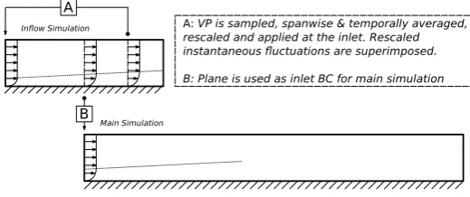
Lundet al. [2] (herein referred to as LWS) developed a quasi-periodic approach utilising an accurate
scaling technique. This method used recycling of the downstream data to provide the inlet boundary condition on the inflow simulation (illustrated in Figure 1). It has been successfully applied in both incompressible and compressible boundary layer simulations [3–5]. Despite the wealth of publications that have successfully applied this method, a number of studies [5–10] have indicated that some aspects of LWS method can prove difficult to implement. Hurdles include spurious periodicity, error accumulation, and initial conditions. The main objective of this Technical Note is to propose simple modification to the original LWS formulation to address these issues, and also to avoid use of the 99% boundary layer thickness (δ).
Figure 1: Recycling inflow generation method.
2
Recycling Inflow Generation Methods
Recycling techniques can be susceptive to non-physical interaction between the downstream recycle plane (where the flow-field is sampled) and the inlet plane (where the rescaled flow field is re-introduced). There is potential for spurious periodicity: streamwise repetition of flow structures, with a wavelength of the order of the distance between the two planes [11, 12]. This amounts to non-physical periodic forcing of the flow [5] and the highly recurrent data could be particularly problematic if their frequency corresponds to a physically relevant one in the flow studied downstream [13]. Simenset al. [10] suggested that eddies in boundary layers can remain coherent for more than 300 momentum thicknesses (θ) downstream, which is much longer than the integral length scale of the turbulent boundary layer.
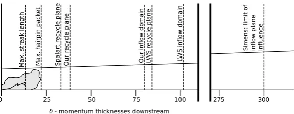
There is also the potential vulnerability of recycling techniques to feedback of error, and this can lead to error accumulation. Particularly when inflow and recycle planes are located close to one another, numerical artifacts can be introduced into the mean flow [10, 14]. Lygren and Andersson [15] observed a non-physical secondary formation of spanwise ‘roll-cells’ in their plane Couette flow simulation. This inflow-outflow coupling is ‘self-amplifying’ and associated with the linking and elongation of coherent structures between planes [16]. Simenset al. [10] also reported that with a recycling plane close to the inflow (4δ0), the entire computational domain was filled with non-physical flow structures, raising the free-stream turbulence level toO(1). Close planes in the boundary layer enable instantaneous streamwise structures to link non-physically. The near-wall streaks extend over a distance of 1000 in wall units: using the flow conditions cited in LWS, this translates to approximately 16θ. Similarly, large-scale hairpin vortex packets extend up to 2.3δ≈23θ [17]. Figure 2 is an illustration of the configuration of various simulations, and the approximate streamwise extent of various instantaneous coherent structures in the boundary layer. It is easy to see how spurious interaction between coherent structures could occur as recycle plane placement moves closer to the inlet. In the following section, simple modification was described to tackle these issues.
Figure 2: Illustration various LWS-based inflow simulation configurations, compared to the lengths of instantaneous boundary layer structures. This illustration is intended to highlight relative scales.
3
Proposed Modification
3.1
Mirroring Method
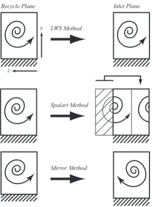
In this study, an inflow disruption method was considered to deal with the spurious feedback behaviour when the recycle plane was placed close to the inlet. Periodic spanwise boundary conditions were applied to disrupt the spurious linking of structures re-applied at the inlet by mirroring the inlet plane. This mirroring technique was successfully used for plane Couette flow [15]. This is designed to avoid spurious linking between planes by removing any streamwise alignment, whilst maintaining realistic coherent structures at the inlet. The concept is illustrated in Figure 3.
From the rescaled inlet velocity field:
u(y, z, t)mirror,in= u(y, W−z, t)in, (1)
v(y, z, t)mirror,in= v(y, W−z, t)in, (2)
w(y, z, t)mirror,in= −w(y, W−z, t)in, (3)
whereu, vandware velocity components in streamwise (x), wall normal (y) and spanwise (z) directions, respectively. W is the domain width, and t is the time. The new mirrored values foru, v and wwere applied at the inlet instead of the originally calculated velocity field. Note that the scheme is consistent and compatible with the spanwise w offset caused by the staggered grid, and also that w has to be negative to ensure spatial coherence once mirrored.
3.2
Use of
δ
∗instead of
δ
Figure 3: Methods for disrupting error accumulation.
stages of the inflow simulation, when the mean profile at the recycle point was still developing. The LWS scheme was reformulated to use an integral measurement, specifically the displacement thickness,δ∗.
In our modification, length scales are non-dimensionalised with respect toδ∗instead ofδ, andη=y/δ∗
is used in the same manner as in LWS. The only equation that requires modification is the weighting function used to blend the inner and outer boundary layer profiles. For this purpose, a seventh power law approximation is used to expressηin terms ofδ(sinceδ∗≈0.125δ). Equation (16) in LWS becomes:
W(η/8) = 1 2
1 + tanh
α(η/8−b)
(1−2b)η/8 +b
tanh(α)
. (4)
Parameters (α and b) remain the same as in LWS, and the equation used to produce the composite velocity profile remains unchanged. An added advantage of basingη onδ∗ was that a very stable inlet mass flux was produced. Iterating the calculation of the inlet flow field to accurately converge onδ∗= 1.0 rather thanδ= 1.0 ensured that the mass flow across the inlet boundary remained constant.
3.3
Initial Conditions
Another issue alluded to in the literature [8–10] is that the initial conditions proposed by LWS are insufficient for the effective initialisation of turbulent flow. For example, Liu and Pletcher [9] observed that poorly posed initial conditions led to the continuous decay of Reynolds stresses (and subsequent re-laminarisation). Various approaches have been suggested for improving the initial conditions. Liu and Pletcher [9] focused on manipulating the starting transients, and opted to implement a dynamic recycle plane method to ensure that the recycle plane moved dynamically downstream from the start of the simulation, such that it was held in within the turbulent region produced by inflow conditions. Attempts were also made to use turbulent kinetic energy spectrum [8] and an accurate DNS flow-field [10] for the
0 10 20 30 40 50 60 3
3.5 4
x
C f
Cf
Cfestimation from 7th power law
location of recycling plane
[image:6.595.187.408.80.276.2]/δ*
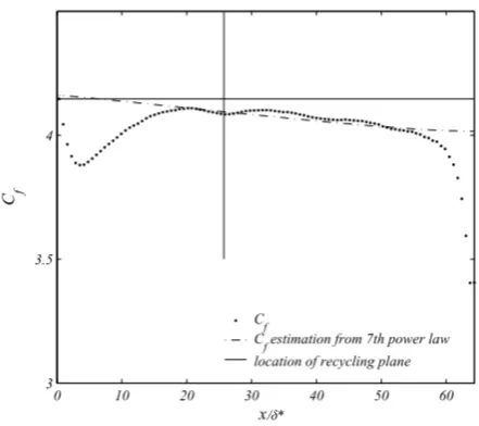
Figure 4: Time and spanwise averaged Cf(×103) in a streamwise direction, with inlet mirroring.
initialisation. Although these methods [8–10] were effective, they added unnecessary complexity to what should be a fairly straightforward problem. Instead, we proposed simple modification to the original initial conditions used in LWS.
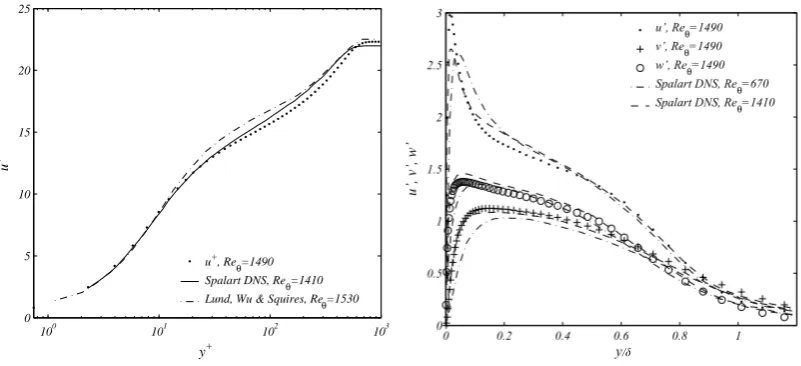
At initialisation, an approximateuvelocity flow field was built around a simple mean profile provided by the Spalding law [18], growing in a streamwise direction, according to the increase inRex, based on the downstream distance. Atyvalues greater thanδthe free-stream velocity was imposed. The random velocity fluctuation intensities (u0, v0 and w0) were stepped to roughly match intensity profiles in the boundary layer [19]; such that the turbulent intensity peaked aty/δ= 0.05, then progressively decayed towards the outer boundary layer (see Figure 5b)). The amplitude of the velocity fluctuations were set as|u0| ≤0.8u, |v0| ≤0.5u, |w0| ≤0.6u for 0.05≤y/δ <0.25. The fluctuations were then reduced by a factor of two in the region 0.25≤y/δ <0.5, and by a factor of four in the region from 0.5 ≤y/δ <1. It should be noted that these inflow conditions were forReδ∗ = 2000 and these weighting values would
vary with the Reynolds number.
4
Results and Discussion
Results presented in this paper have been computed using a second-order finite-volume code [1, 20]. The convective terms were modelled using a third order Runge-Kutta method, and the diffusive terms using a Crank-Nicolson method. A dynamic Smagorinsky subgrid-scale model [21] was used. TheRenumber based on the inlet displacement thickness (δ∗in) and the free-stream velocity (U∞) isReδ∗= 1800. The
inflow simulation domain had dimensions 64δ∗
in×24δin∗ ×4πδin∗ , with a corresponding grid density of
100 101 102 103 0 5 10 15 20 25 y+ u +
u+, Re
θ=1490
Spalart DNS, Re
θ=1410
Lund, Wu & Squires, Re
θ=1530
0 0.2 0.4 0.6 0.8 1
0 0.5 1 1.5 2 2.5 3 y
u’, v’, w’
u’, Reθ=1490 v’, Reθ=1490 w’, Reθ=1490 Spalart DNS, Reθ=670 Spalart DNS, Reθ=1410
[image:7.595.99.500.73.256.2]/δ
Figure 5: Time and spanwise-averaged data for Reθ = 1490: (a) mean velocity profile; (b) velocity fluctuation profile.
this yielded a mesh resolution, ∆x+ ≈ 59, ∆y+wall ≈ 1.2, and ∆z+ ≈ 18. The domain size and the resolution were similar to those used in LWS. The boundary conditions at the upper boundary of the domain wereu=U∞, ∂v∂y = 0, ∂w∂y = 0, and the exit plane used a convective boundary condition.
4.1
Interaction between the inlet and recycle planes
Figure 4 shows the time and spanwise averaged skin friction coefficient, Cf. The spanwise mirroring
causes a small decrease in the skin-friction near the inlet, and this is due to the disruption of near-wall structures by the mirrored inlet plane. Cfrecovers the equilibrium flat-plate boundary layer values within
two to threeδ, so that the recycle plane for the inflow boundary condition can be located downstream from x/δ∗ ≈ 20. Sagaut [22] suggested that the transitional length is proportional to δ. It would be interesting to see how the transitional length changes with the Re number. However, this was not considered here. Figure 4 shows that the spanwise mirroring used in this study is effective in preventing spurious feedback of error, while allowing a quick recovery to the equilibrium boundary layer. With mirroring, it was possible to move the recycle plane to a position very close to the inlet (see Figure 2) using a less computationally costly inflow simulation.
The sample plane for the main simulation inflow was then taken from a well-resolved position down-stream of the recycle plane. This is different to the original LWS method, where the main simulation inflow was sampled from a position between the inflow and recycle planes. It is found that the down-stream development of the velocity field agrees well with the boundary layer theory. The mean velocity as well as the velocity fluctuation profiles at Reδ∗ = 1910 (corresponding to Reθ = 1490) are shown
in Figure 5. They show good agreement with Spalart DNS data [19]and LWS data [2] at similar Re
numbers.
0.020 0.025 0.030 0.035 0.040 0.045 0.050 0.055
0 200 400 600 800 1000 1200 1400
Shear Velocity, u
τ
Time, t
[image:8.595.184.419.73.295.2]Original Revised
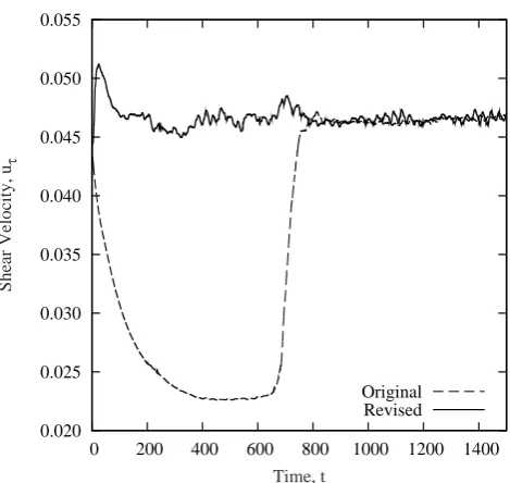
Figure 6: Development of uτ over time at the inlet; original vs revised initial conditions.
4.2
Initial Conditions
Figure 6 shows the time history of friction velocity,uτ, at the inlet plane. The original LWS conditions resulted in a large starting transient: the initial reduction in friction velocity using LWS method indicates relaminarisation, followed by eventual transition to turbulent flow. On the other hand, no evidence of relaminarisation is shown with our method, indicating that our simple modification to the LWS initial conditions was sufficient to quickly initialise a turbulent boundary layer, without any undesirable relaminarisation behaviour.
5
Conclusions
Acknowledgments
This work was supported by the Engineering and Physical Sciences Research Council through the UK Turbulence Consortium (Grant EP/G069581/1).
References
[1] Y. M. Chung and H. J. Sung. Comparative study of inflow conditions for spatially-evolving simu-lation. AIAA Journal, 35(2):269–274, 1997.
[2] T. S. Lund, X. Wu, and K. D. Squires. Generation of turbulent inflow data for spatially-developing boundary layer simulations. Journal of Computational Physics, 140(2):233–258, 1988.
[3] S. Kang and H. Choi. Suboptimal feedback control of turbulent flow over a backward facing step.
Journal of Fluid Mechanics, 463:201–227, 2002.
[4] C. Dimitropoulos, Y. Dubief, E. Shaqfeh, P. Moin, and S. Lele. Direct numerical simulation of polymer-induced drag reduction in turbulent boundary layer flow. Physics of Fluids, 17:011705, 2005.
[5] E. Garnier, N. Adams, and P. Sagaut. Large Eddy Simulation for Compressible Flows. Springer, 2009.
[6] M. Klein, A. Sadiki, and J. Janicka. A digital filter based generation of inflow data for spatially devel-oping direct numerical or large eddy simulations.Journal of Computational Physics, 186(2):652–665, 2003.
[7] A. Keating, U. Piomelli, and E. Balaras. A priori and a posteriori tests of inflow conditions for large-eddy simulations. Physics of Fluids, 16(12):4696–4712, 2004.
[8] A. Ferrante and S. E. Elghobashi. A robust method for generating inflow conditions for direct simulations of spatially-developing turbulent boundary layers. Journal of Computational Physics, 198(1):372–387, 2004.
[9] K. Liu and R. Pletcher. Inflow conditions for the large eddy simulation of turbulent boundary layers: A dynamic recycling procedure. Journal of Computational Physics, 219:1–6, 2006.
[10] M. Simens, J. Jiminez, S. Hoyas, and Y. Mizuno. A high-resolution code for turbulent boundary layers. Journal of Computational Physics, 228(11):4218–4231, 2009.
[11] A. Spille-Kohoff and H. Kaltenbach. Generation of turbulent inflow data with a prescribed shear-stress profile. In3rd ASOFR International Conference on DNS/LES, Arlington, TX, 2001. [12] N. Nikitin. Spatial periodicity of spatially evolving turbulent flow caused by inflow boundary
con-dition. Physics of Fluids, 19:091703, 2007.
[13] M. Pami`es, P.- ´E. Weiss, E. Garnier, S. Deck, and P. Sagaut. Generation of synthetic turbulent inflow data for large eddy simulation of spatially-evolving wall-bounded flows. Physics of Fluids, 21:045103, 2009.
[14] P. R. Spalart, M. Strelets, and A. Travin. Direct numerical simulation of large-eddy-break-up devices in a boundary layer. International Journal of Heat and Fluid Flow, 27:902–910, 2006.
[15] M. Lygren and H. Andersson. Influence of boundary conditions on the large-scale structures in turbulent plane couette flow. In S. Banerjee and J. K. Eaton, editors,Turbulence and Shear Flow
Phenomena -1, volume 1, pages 15–20. Begell House, 1999.
[16] H. Andersson, M. Lygren, and R. Kristofferson. Roll cells in turbulent plane couette flow: Reality or artifact? In16th International Conference on Numerical Methods in Fluid Dynamics, 1998. [17] R. Adrian, C. Meinhart, and C. D. Tompkins. Vortex organisation in the outer region of the
turbulent boundary layer. Journal of Fluid Mechanics, 422:1–54, 2000.
[18] D. B. Spalding. A single formula for the law of the wall. Journal of Applied Mechanics, 28:455–458, 1961.
[19] P. R. Spalart. Direct simulation of a turbulent boundary layer up to θ = 1410. Journal of Fluid
Mechanics, 187:61–98, 1988.
[20] Y. M. Chung and H. J. Sung. Initial relaxation of spatially evolving turbulent channel flow subjected to wall blowing and suction. AIAA Journal, 39(11):2091–2099, 2001.
[21] M. Germano, U. Piomelli, P. Moin, and W. H. Cabot. A dynamic subgrid-scale eddy viscosity model. Physics of Fluids A, 3(7):1760–1765, 1991.