Bayesian inference on non stationary data

warwick.ac.uk/lib-publications

A Thesis Submitted for the Degree of PhD at the University of Warwick

Permanent WRAP URL:

http://wrap.warwick.ac.uk/109025

Copyright and reuse:

This thesis is made available online and is protected by original copyright.

Please scroll down to view the document itself.

Please refer to the repository record for this item for information to help you to cite it.

Our policy information is available from the repository home page.

THE BRITISH LIBRARY

BRITISH THESIS SERVICE

TITLE

BAYESIAN INFERENCE ON NON-STATIONARY

_DATA

AUTHOR

Giovanni

AMISANO

DEGREE

PhD

AWARDING

Warwick University

BODY

DATE

1995

THESIS

DX193331

NUMBER

THIS THESIS HAS BEEN MICROFILMED EXACTLY AS RECEIVED

The quality of this reproduction is dependent upon the quality of the original thesis submitted for microfilming. Every effort has been made to ensure the highest quality of reproduction. Some pages may have indistinct print, especially if the original papers were poorly produced or if awarding body sent an inferior copy. If pages are missing, please contact the awarding body which granted the degree.

Previously copyrighted materials (journals articles, published texts etc.) are not filmed.

This copy of the thesis has been supplied on condition that anyone who consults it is understood to recognise that it's copyright rests with its author and that no information derived from it may be published without the author's prior written consent.

BAYESIAN INFERENCE ON

NON-STATIONARY DATA

Giovanni Amisano

Department o f Economics,

University o f Warwick

September 1995

To my parents with love and gratitude

Two roads diverged in the yellow wood,

and I,

I took the road less traveled by

Table of Contents:

Acknowledgements v

Summary vi

Chapter 1: Introduction and Outline I PART I: The Univariate Analysis of Non-Stationary Time Series 7 Chapter 2: The Frequentisi Approach to Non-stationarity in univariate 7

Time Series Analysis

[2 0] An Overview of the Chapter 7

[2.1] Integrated versus trend stationary processes 7

[2.2] Inference on trend stationary and integrated univariate processes 13

[2.3] Some General Considerations About Unit Root Testing in a 25

Classical Framework

Chapter 3: The Bayesian Approach to Time Series Analysis: 28 Problems and Methods.

[3.0] An Overview of the Chapter 28

[3.1] General Philosophy o f the Bayesian Approach 28

[3.2] Bayesian Inferential Techniques 33

[3.3] The specification of the priors 40

[3.4] Computational Problems and Technical Solutions 46

[3.4. a] Approximations 47

[3 4.b] Numerical integration 48

[3.4.c] Monte Carlo Integration and Importance Sampling 49

[3.4.d] Markov Chain Monte Carlo: Gibbs Sampling and Metropolis- 56

Hastings Algorithms

[3 .4.e] Measuring the accuracy o f MC Monte Carlo estimates 63

1 [3 6] Ignorance Priors in Time Series Models 74

C hapter 4: Bayesian Analysis of Integration a t Different Frequencies in 78

Q uarterly D ata

[4 0] An Overview of the Chapter 78

[4 .1] General Features of the Model 80

[4.2] The Specification of the Priors 84

[4.3] The Joint Posterior Distribution 87

[4 4] The conditional posterior distributions 90

[4.5] A Convenient Description of the Posterior Odds Ratio 91

[4.6] An Application 97

[4.7] Conclusion 105

Appendix [4. A]: Proofs of distributional results 105

Appendix [4 B] : Rejection Sampling from the Conditional Posterior 110

Distributions

Appendix [4.C] : Proofs of the Smooth Transition Results 113

PART II: The Multivariate Analysis of Non Stationary Time Series 120

Chapter 5: Non Stationarity in Multivariate Time Series Analysis. 120

The Classical Approach

[5.0] An Overview of the Chapter 120

#

[5.1] Spurious Regression and Cointegration 121

[5.2] Representation and identification issues 123

[5.3] Estimation Issues 128

[5.4] Interpretation of the Cointegrating Coefficients 136

[5.5] Asymptotic Distributions of the Parameter Estimates 139

Chapter 6: Bayesian Inference in Cointegrated Systems 145

[6 0] An Overview o f the Chapter 145

[6.1] Motivations 146

[6.2] The Model 148

[6.3] The Prior Distribution 150

[6 4] The Joint Posterior Distribution 152

[6.5] Inference on Cointegration Rank 159

[6 6] Testing Restrictions on the Cointegration Space 162

[6 7] Some Applications 165

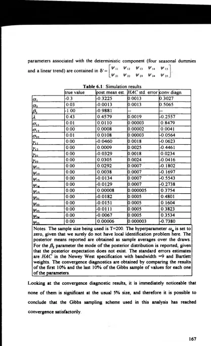
[6.7.1] A simulated data set example 166

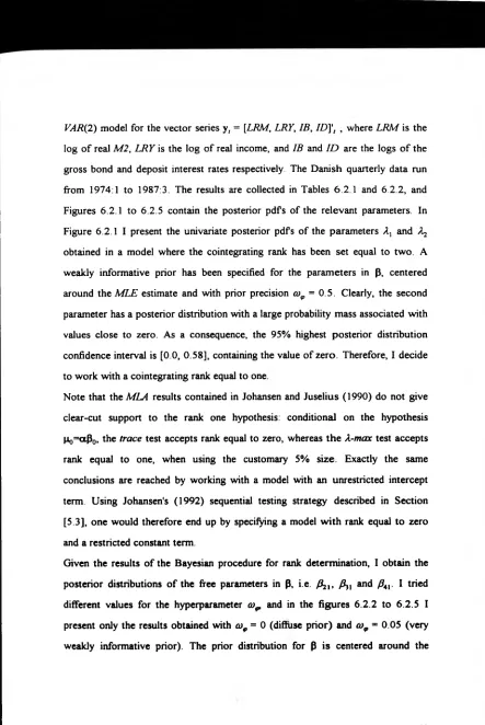
[6.7.2] The Danish Money Demand Example 168

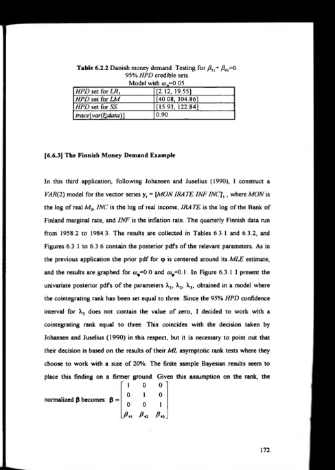
[6 7.3] The Finnish Money Demand Example 172

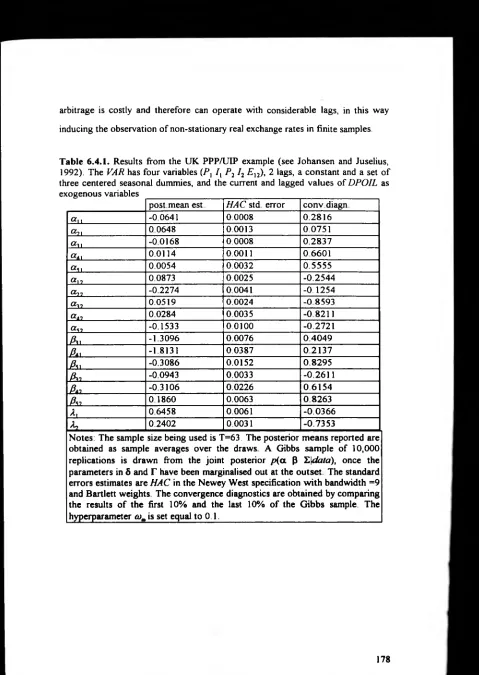
[6.7 4] The UK PPP/UIP Example 175

[6 8] Conclusion 179

Chapter 7: Concluding remarks 191

References 196

List of tables and illustrations

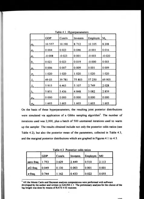
Table 4 1 100

Table 4.2 100

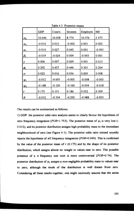
Table 4.3 101

Table 4 4 104

Figure 4 1 115

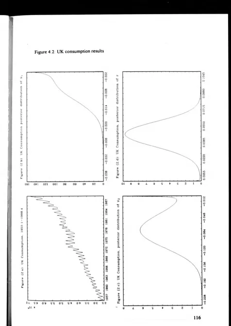
Figure 4.2 116

Figure 4 3 117

Figure 4 4 118

Figure 4 5 119

Table 6.2.1 171

Table 6.2.2 172

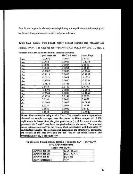
Table 6 3.1 174

Table 6.3.2 174

Table 6 4 1 178

Table 6.4.2 179

Figure 6.2 1 180

Figure 6.2.2 180

Figure 6.2.3 181

Figure 6.2 4 181

Figure 6.2.5 182

Figure 6.3.1 182

Figure 6.3.2 183

Figure 6 3.3 183

Figure 6.3 4 184

Figure 6 3.5 184

Figure 6.3 6 185

Figure 6 4 1 185

Figure 6 4.2 186

Figure 6 4.3 186

Figure 6 4 4 187

Figure 6 4.5 187

Figure 6.4.6 188

Figure 6.4.7 188

Figure 6.4 8 189

Figure 6 4 9 189

Figure 6.4.10 190

Aknowledgments

I would like to express my sincere gratitude to all the people I bothered with my

questions I greatly benefitted from discussions with Rocco Mosconi, Mario

Seghelini, Jeremy Smith and Sanjay Yadav I also received valuable suggestions

from Frank Kleibergen, John Geweke and Hermann van Dijk at different stages of

my work.

Carlo Giannini deserves all my gratitude for having been my first and great

econometrics teacher He started me off as an econometrician, encouraged me to

go and study abroad, and gave me constant scientific inspiration throughout my

career Grazie Carlo, sei un fra tello

Kenneth Wallis, my supervisor, let me have the benefit of all his experience and

competence, and gave me his warm encouragement in several difficult stages in the

preparation of this thesis I sincerely thank him for that, and I apologise for having

so often tested his infinite patience

The only non-econometrician person to appear in this list is my wife Anne who did

not know what "Bayesian" and "unit root" meant before she met me I am not sure

Summary

This thesis argues in fa vo u r o f Bayesian techniques fo r the analysis o f non-stationary linear time series. The main motivations are to avoid using asymptotic results and to explicitly incorporate prior beliefs, where they exist.

The properties o f univariate and multivariate unit root models, and the available frequentist inferential results are described. Some problem s in their applications are highlighted: the discrepancies between asym ptotic and fin ite sample properties and the role o f the determ inistic components in determ ining the reference asymptotic distributions.

The advantages and disadvantages o f Bayesian techniques are then examined with the recent developments in the M onte Carlo integration by M arkov Chain sampling. Two case studies are conducted with the aim o f providing evidence o f the applicability o f Bayesian techniques.

The fir s t o f these cases develops a procedure to test fo r seasonal and/or zero frequency unit roots in quarterly series. A new param eterisation is provided and the priors implemented are discussed and justified. The analysis relies on a Gibbs sam pling scheme. The inferential technique used is the evaluation o f posterior odds ratios. These ratios are defined as posterior expectations o f functions o f the parameters, and therefore can be consistently estim ated The procedure is applied to some UK variables. The results are robust w ith respect to different prior distributions, and conflict w ith some conclusions reached by using classical asym ptotic unit root tests.

The second case study develops a Bayesian procedure to conduct inference in cointegrated systems. Inference regards the number o f cointegrating relationships and their structural interpretation, and is based on the evaluation o f highest posterior density confidence intervals.

Chapter 1: Introduction and Outline

Weakly stationarity processes, processes whose first and second order moments

do not vary over time, have played a central role in the traditional econometric

analysis o f linear time series data Unfortunately, assumptions o f constancy of

moments seem at odds with most observed economic time series.

Different alternative models o f non-stationarity behaviour have been proposed,

implying radically different long-run properties for the series under study. A simple

way to account for non-stationarity is to assume that the process is stationary

around a deterministic trend. Such a process has constant second order moments

and shocks have only a transitory effect on it. Alternatively, it is very often

assumed that one or more unit roots are present in the autoregressive

representation. A unit root process is characterised by a growing variance, and by

the fact that shocks have a permanent effect on the level o f the series

Economic theory has provided models implying the presence of unit roots in many

macroeconomic aggregates. General equilibrium business cycle models emphasise

the role o f persistent shocks Intertemporal quadratic utility maximisation leads to

non-stationarity for individual consumption The efficient market hypothesis

implies an exploding variance for the asset price forecast error, as the forecasting

horizon grows.

In the last two decades the statistical analysis of linear time series has made

enormous progress by providing the researcher with the technical tools necessary

to deal with unit root processes, and to discriminate between different models of

non-stationarity The asymptotic distributions o f the parameters estimates for unit

root autoregressive processes have been thoroughly investigated and some

First of all, these distributions are non-standard, since they are complicated

functionals of Brownian motion processes The exact form of these functionals

depends on which deterministic components are included in the estimated model

and in the true data generation mechanism. On the basis of these new asymptotic

results, some testing procedures have been developed to ascertain the presence of

unit roots in observed time series and therefore to discriminate between competing

models o f non-stationary behaviour.

As in the analysis of the long-run properties of univariate processes, also the

phenomenon o f seasonality can be explained on the basis o f different competing

models A first possibility is to account for seasonality by introducing a set of

seasonal dummy variables A second possibility is that unit roots at seasonal

frequencies are present in the autoregressive polynomial This particular form of

seasonality requires the application of an adequate filter to induce stationarity and

raises the issue o f the occurrence of common stochastic seasonality patterns in

multivariate time series Seasonal unit root tests have been developed, in order to

discriminate between competing ways to model seasonality As the zero-frequency

unit root tests, these testing procedures are based on non-standard asymptotic

distributional results

In the analysis o f multivariate time series, the problem o f the interpretation of

results o f regressions among non-stationary variables is directly connected to the

"spurious regression" problem The notion of spurious regression relates to a

regression among non stationary variables, when good measures of fit may be

found even in the absence of any direct links among the variables

In many cases, though, true long-run relationships do exist among non-stationary

variables Long-run relationships are particularly interesting because they relate to

the notion of equilibrium links among sets of economic variables The widely

popular concept o f cointegration directly refers to the existence o f long-run

long-run multipliers in the autoregressive representation o f a vector series. The rank of

this matrix gives the number of stationary variables generated as independent linear

combinations of the non-stationary series being considered Each one of these

stationary variables can be interpreted as deviations from a corresponding long-run

relationship

During the last few years, new inferential techniques have been proposed in order

to analyse potentially cointegrated vector series Inference mainly regards the

number of cointegrating relationships and their structural interpretation as

equilibrium relationships The asymptotic distributional properties of estimators

and testing procedures being used in this regard are again non-standard and depend

on which deterministic components are thought to be present in the 'true' data

generation process

In synthesis, the analysis of univariate and multivariate inferential properties of unit

root processes led to a great advancement in the statistical foundations of

econometric modelling, allowing proper treatment o f non-stationary data

Unfortunately, these new inferential results present the applied researcher with

some unpleasant features Many Monte Carlo studies have revealed that the finite

sample inferential properties of non-stationary models can be radically different to

their known asymptotic counterparts In most macroeconometric applications,

where the typical sample size is well below 100 observations, reliance on

inappropriate inferential results is extremely likely In addition, the sensitivity o f the

scaled asymptotic distribution to the deterministic part o f the model causes further

complications, since the researcher cannot be sure about the correctness o f the

model specification in this regard

Moreover, it is evident that the finite sample behaviour of observed series can be

explained almost equally well by unit root and by stationary near-unit root

processes This problem o f observational equivalence clearly generates very bad

For these reasons, recent contributions in the analysis of non-stationary series have

suggested that resorting to a Bayesian inferential framework could yield more

sensible results.

Bayesian analysis presents three main advantages First of all, uncertainty about the

parameters can be directly measured on the basis o f their posterior distributions,

and no reference to asymptotic results is ever necessary Secondly, a Bayesian

approach requires a clear statement of the researcher's beliefs, in the form o f the

specification o f a prior distribution for the parameters This does not happen in

applications of the frequentist inferential procedures, where prior beliefs, though

unstated, are often incorporated Thirdly, unlike the classical Neyman-Pearson

apparatus, Bayesian model selection techniques are fully consistent, since the

probabilities o f picking a wrong model go to zero as more sample information

becomes available

On the other hand, Bayesian methods present two primary disadvantages The first

one is related to the necessity of providing a prior distribution While most

Bayesian researchers agree on the irrelevance of the issue of how to represent prior

ignorance, a central problem in Bayesian analysis is how to render results

universally acceptable, although they are clearly based on personal convictions

The second disadvantage is a computational one In fact, the typical results of

Bayesian analysis can be defined as posterior expectations o f certain functions o f

interest, these functions need to be integrated with respect to the posterior

probability density function Excluding only a narrow class of cases, this

integration is almost always analytically unfeasible

A satisfactory way of overcoming the first disadvantage is to assess the sensitivity

of the results with respect to the choice o f the prior distribution This can be done

by providing results corresponding to different alternative priors

As for the computational difficulties, the Monte Carlo principle can be used to

consistent estimates of the posterior expectations being studied, but in this context

"consistency" refers to the number of steps in the simulations, which can be as high

as desired, and not to the sample size which is seldom the result of the researcher's

choice

The main problem is then that of efficiently simulating the relevant posterior

distributions, and this goal can be satisfactorily achieved in most econometric

applications by using Markov chain sampling schemes

This dissertation intends to provide examples o f how Bayesian analysis can be

efficiently used to conduct inference on non-stationary series These examples take

the form o f new applications of posterior inference techniques to series which

potentially have unit roots The thesis deals with both univariate and multivariate

issues and is structured as follows

Chapter 2 explains the different properties o f unit root and trend stationary

univariate processes, reviews the frequentist inferential results available for

univariate unit root process, and discusses the properties o f the main testing

procedures to discriminate between the two competing ways to account for non-

stationarity

In Chapter 3 the main characteristics of the Bayesian methodology are examined

Computational problems and technical solutions are discussed at length, with

special emphasis on Markov chain Monte Carlo methods. The literature on the

application o f Bayesian inferential techniques on unit root processes is surveyed

Chapter 4 describes a Bayesian inferential methodology to test for the presence o f

unit roots at seasonal frequencies The technique is based on the evaluation o f

posterior odds ratios by means of a Gibbs sampling scheme. An application on a

set o f UK series is presented

Chapter 5 discusses the problems of how to determine the number of cointegrating

based on maximum likelihood estimation are discussed together with their

asymptotic and finite sample performances.

Chapter 6 describes a Bayesian procedure to test for the cointegrating rank based

on a Gibbs sampling scheme Having determined the rank, other Bayesian

procedures are proposed to test for the over-identifying restrictions on the

cointegration space Some applications are presented on money demand and

exchange rate examples

Chapter 7 contains some conclusive considerations on the evidence gathered in this

PART I: The Univariate Analysis o f Non-Stationary Time Series

Chapter 2: The Frequentist Approach to Non-stationarity in univariate Time Series Analysis.

(2.0] An Overview of the Chapter.

This chapter contains an overview o f the issue o f non-stationarity in univariate

models as seen from a frequentist point of view. In the first section the concepts of

trend and difference stationary processes are introduced, and their different

modelling properties are highlighted In Section [2 2], I describe the existing

inferential procedures designed to detect the presence of unit roots Section [2.3]

contains a brief summary of the main problems encountered in using the techniques

surveyed in the previous section, and provides the main motivations supporting the

adoption o f a Bayesian inferential strategy

[2.1] Integrated versus trend stationary processes.

Many macroeconomic time series show evident trending patterns The theoretical

justification for such non-stationary behaviour is often related to the occurrence of

phenomena like technological progress, increases in population and in the capital

stock, in short to all the forces supposed to drive the key economic variables over

time in the long run. However, the tools o f time series analysis are mainly based on

the assumption o f weak stationarity of the series under study, that is, the

assumption that first and second order moments are time-invariant Therefore, how

to deal properly with the observed non-stationarity is an important question, and

simple and straightforward procedure could be to assume the presence of a

deterministic trend, and detrend the data accordingly by means of a simple

regression, having performed such a transformation, one could then focus on the

resulting series and model the remaining dynamics by means of the available

techniques that rely on stationarity Thus, it is implicitly assumed that the series is

affected by a steady growth pattern, around which it fluctuates due to the

transitory effects of disturbances. Such series is said to be 'trend stationary', i.e to

possess a stationary invertible ARMA representation once the trend has been

removed In the case of a linear trend, we have

A L K y . - n - S t) = % L ) e , (1)

where e, is i.i.d. distributed with mean 0 and variance <re2, and p (L) and 6 (L) are

respectively stationary and invertible, thus in particular y, - p- S t has bounded

variance.

In this framework, the long run is accounted for in a completely deterministic way

(i.e. it is predictable with zero error), and what remains is produced as the dynamic

response to the realisation o f a series o f random disturbances These shocks have

an effect that vanishes in the long run. In fact, the zero-mean stationary process z,

= y , - p - S t admits a Old representation:

z, = [ ^ L ) l f K L ) ] e , = c ( L ) e „

Z c 2 < 00.

J-0

(

2

Given the square summability of MA coefficients for a stationary process, we see

that the effect of a random shock on the levels of the series tends to vanish as time

(3)

lim [àyl+kl â e , ] - lim ck - 0. k-> « k-+<x>

The above quantity measures the persistence of the shocks hitting the series. Such

disturbances can be taken to reflect , in a highly stylised way, the occurrence of

demand side shocks, which induce the observed series to deviate temporarily from

its long run fundamentals (technological progress, demographic factors,

accumulation) driving it along its steady-state path As in Blanchard and Fischer

(1989, p 8), the model can be intended as a canonical form, in which the single

stochastic term is taken to represent the action o f a plurality o f random shocks

This is coherent with the analysis of Granger and Morris (1976)

Secondly, it is possible to conceive o f the observed series as generated by the

cumulated ever-lasting effects of purely random shocks This hypothesis has found

technical justification in the Box-Jenkins ARIMA modelling framework, where it is

recommended that the series be differenced until stationarity is achieved This

means that in the proposed ARM A(p,q) representation:

the autoregressive polynomial, p (Z,), is supposed to have d unit roots, hence once

the series has been differenced d times, y, admits ARM A(p’,q) representation

with p ’ - p - d The original series is then called difference stationary', or to

possess d unit roots in its autoregressive polynomial

If attention is restricted to first differencing, as seems to be plausible for many

macroeconomic aggregates, then we have a stationary ARMA model for the first

differences:

P(L)y, = 0 ( L ) e, (4)

The series is called integrated of order one. As Beveridge and Nelson (1981) show,

any such process can be decomposed into two different random components, the

first being a random walk with drift , and the second a stationary zero-mean

ARMA process:

y, = y f ’ + y!>

Ay; = 5 + k l ) / p ( l ) k = S + c ( l ) e „

.

y, = c (L)e, ,

c(L) = [fl(L)/p*(L)] = c'(Z )A + C(l).

The drift arises only if the differenced process has a non-zero mean The first

component can be interpreted as accounting for the growth of the process: its

differences deviate randomly from the non-zero expected value given by the drift,

with a variance which is [c(\)]2ae2 The second component gives the transient

short run dynamics In this model shock have an ever-lasting effect on the level of

the series given by a non-zero persistence measure:

lim [ à y , ^ t de, \ = c(l) * 0.

k-* oo (7)

A synthetic measure of the importance o f the non-stationary component y , is

therefore given by the sheer size of c(l), which is a non-linear function o f the

parameters of the AR and MA coefficients

Note however that both components are by definition generated in terms of the

same random disturbance term ep hence the long run and transitory dynamics

cannot be considered as distinct, and the shocks affect the variable in a permanent

way through their effect on y , This is just one of the possible decompositions

decomposition in terms of different orthogonal processes, which forms the basis of

the ' structural time series modelling1.

Models like (6), when applied to variables such as gnp or its components, are

compatible with a very different explanation o f the observed fluctuations, namely

that provided by the "real business cycle" theory. See, for example, Plosser (1982),

Kydland and Prescott (1982), Prescott (1986), King, Plosser and Rebelo (1988),

Campbell (1994) In such a theoretical framework, the role of inter-temporal

optimising behaviour o f rational agents in labour-leisure and consumption-

investment choices is emphasised, and shocks from different sources are allowed to

produce permanent effects on the series itself, by modifying its random growth

pattern These shocks are mainly, but not only technological: disturbances can

affect tastes and preferences, and can take the form of public sector interventions

(see Baxter and King, 1993 or Campbell 1994), or of unexpected changes in the

terms of trade (as in Mendoza 1991, or Correia et al. 1995). It is not even

necessary that such shocks be given a non-stationary specification to produce

permanent effects, given the inter-temporal capital accumulation process In the

short run, the occurrence of disturbances produces temporary effects through the

adjustment mechanism, which are intended to be accommodated in the second term

o f the above decomposition Moreover such short-run disturbances are part o f the

optimal reaction of economic agents For this reason they should be considered as

Pareto optimal and not as something the government should aim at offsetting This

is not the only possible explanation o f the occurrence o f persistent shocks, and its

validity is strongly questioned (see Mankiw, 1989). Campbell and Mankiw (1987)

regard this persistence as better explained by the presence o f nominal rigidities or

by multiple equilibria.

In many other fields of economic analysis recent theories imply difference

the presence o f a unit root is often a theoretical im plication o f m odels which

postulate the rational use o f information available to economic agents. Examples

from economics include various financial market variables, such as future

contracts [...], dividends and earnings [...], spot and forw ard exchange rates [...],

and even aggregate variables like real consumption [...] and investment

(Perron (1988, p.297)

From a more technical viewpoint, in the recent methodological literature it has

been emphasised that the correct starting step in econometric modelling is a well

defined estimated statistical model (Spanos, 1986)' to account for the statistical

properties of the series under study Therefore, it is important to discriminate

between the two kinds of non-stationarity at the outset, also in the light of the

impact on properties of estimators

In many studies, e g Phillips and Durlauf (1986), Park and Phillips (1988) and

(1989), West (1988) and Sims, Stock and Watson (1990) inter alia, properties of

estimators have been analysed in regression contexts where some o f (or all) the

variables involved are integrated In such cases, estimators may not have

asymptotic normal distributions, and they usually do not have Therefore all the

tests that are commonly used in regression analysis have asymptotic distributions

which deviate from the usual %2, and need numerical tabulation

For all these reasons a host o f applied studies have been conducted on a univariate

basis, to discriminate between trend and difference stationarity The first and most

influential paper in that respect is Nelson and Plosser (1982), where most of the

U S. macroeconomic variables considered have been found integrated o f order one

The technical instruments used there are the usual unit root tests put forward by

D A Dickey and W A. Fuller, which are discussed in the following section, after

providing an overview of the properties of the OLS estimates in the trend

[2.2] Inference on trend stationary and integrated univariate processes.

Let us consider a simple zero-mean first order autoregressive process:

y, = p y,-\+ e, .

e, ~i.i.d.(0,cr2). (8)

Clearly, when |p| < 1 the model is an extremely simple stationary process, with

stationary oscillations around its zero unconditional mean The dynamic effect of

shocks can be described via the moving average representation

y, = c(L)e, ,

c, = 0 , i = 1, 2, (9)

Being given a sample of T+1 observations, .y0, y x, ..., y T, the simplest way to

estimate the unknown parameters o f the above process is to use ordinary least

squares, which entails maximising the likelihood conditioned on the initial

observation y 0:

T

j j.

p = '-'r ' ' , a 2 =(T-\y'j^(y, - p y,_,)2 (10)

zx.

It is well known, since the work by Mann and Wald (1943), that the asymptotic

distribution o f the normalised estimate is normal:

7"/J( p - p ) i t f [ 0 , ( 1 - p 2)] (11)

Therefore, given the sample size, the precision of the estimate of p is an increasing

drawn from a different viewpoint, which will be become relevant in the next

chapter. Assuming that the error terms are Gaussian, the conditional log-likelihood

function of the model, reads:

(12)

The Fisher information matrix I T(b) is:

/j.(b) = [ - £ ( ^ log L/i?b<?b')] = 77 2o-4 0

0

T / ( \ - p 2) (13)

Given the notorious equivalence o f the OLS and the conditional ML estimators,

and the usual asymptotic properties of the latter one, the second diagonal element

o f the information matrix conveys immediately the Mann and Wald (1943) result

Nevertheless, it is important to stress that in finite samples the shape o f the

distribution o f p is very different from normal, being skewed to the left, the

skewness being an increasing function of the true unknown value o f p

A generalisation of result (11) holds for the estimation of a stationary AR (p)

process:

y, = p,y,-i + py,.2 + + p? ,.p + £r ( 14)

stating that the scaled OLS estimate of p = [p,, p^, .... pp]' is asymptotically

(15)

7”'2(p- P)4 n[o, ct2V' ] ,

V = varf^,,, y,_2 y,_p]

Therefore, also for higher order stationary AR processes, inference can be

conducted by using asymptotic normality.

Furthermore, if the stationary model is augmented to include a linear time trend:

y, = a + P t + p,y,_, + pyyu2 + ... + pjy,_p + e, (16)

the scaled OLS estimator of b = [p', a, p ]' is asymptotically multivariate Normal:

Tj.(b-b)^>N [o,

---1

< o o

_{__}

V ‘ = 0 1 1/2 II O In M O

0 1/2 1/3 0 0 T in

V = var[z,_, z,_2 ',2, =y, - a - f i t .

Note that the trend term o f the deterministic component has a higher rate of

convergence than the other coefficients and this circumstance calls for the use of

different scaling factors through the apt definition o f the scaling matrix T r (see

Sims, Stock and Watson 1990).

Given the distributional results described above, it is possible to make standard

inference on the parameters o f a stationary AR process Things seem to radically

change when dealing with processes with a unit root. In the case the process is

difference stationary, radically different properties attain for the parameters

estimates. Early studies in this respect are Fuller (1976), Dickey (1976), Dickey

and Fuller (1979, 1981) More recently Phillips (1987) has given a more formal

description o f these properties by making extensive use o f the functional central

Let us consider the simple model (8) where the true value of p is unity. In order to

describe the asymptotic properties o f the OLS estimate of p, it is necessary to

define:

[ Tr]

ST(r)= 2 e„ r e [ 0 ,l] , Sr (r): [0 ,l]-> R , (18)

with [T r] denoting the integer part of T r. A very useful result is what in the

literature is termed as "Donsker's theorem", or "functional central limit theorem",

or "invariance principle" (see Billingsley 1968), stating that:

r ina ' S T(r)=>W(r), (]9 )

where the random variable W (r) is a Brownian motion process, and => denotes

weak convergence of the associated probability measure, this property is the

analogue of convergence in distribution as applied to function spaces It is possible

to see that this result holds also in the presence o f less strict requirements for the

error terms ep for instance when there is some correlation and time-heterogeneity

among them, and this is used in Phillips (1987). Expression (19) states the

asymptotic normality of any normalised sample mean obtained by making use of

sub-sets of the sample observations For instance, when r =1, S ^ l ) is the

normalised sample mean obtained using the full sample, whose asymptotic

distribution is clearly A (0,1), and it is known that this is indeed the distribution of

W(\). In other terms (18) is a more general statement of the central limit theorem

A second very useful result is given by the "continuous mapping theorem", (Hall

and Heyde, 1980) stating that if S ^ r ) converges to S, and g(Sj(r)) is a continuous

functional, then g(Sj(r)) converges to g(S).

Given these results, it is possible to obtain the asymptotic distribution o f the

(20)

0

It is necessary to stress some features of the distribution above, contrasted to the

ones of the analogue asymptotic distribution in the case of stationarity. First of all,

in order to have a non-degenerate distribution, it is necessary to scale ( p -1) by T

and not by P a as in the stationary case In other terms p is Op(T) and not

0,(7™ ). Secondly, although the finite sample distribution o f p is skewed both

under the stationary and the integrated case, in the latter case the asymptotic

distribution o f the adequately normalised bias retains its skewness, whereas it is

Gaussian in the former case

On the basis of the continuous mapping theorem, also the asymptotic distribution

of the t statistic for testing the presence of a unit root can be directly obtained

The random variables defined in the expressions (20) and (21) can be simulated

and therefore it is possible to obtain the desired quantiles Tables for both statistics

are contained in Fuller (1976, p 371). Together with the asymptotic quantiles,

Fuller provides also the quantiles for different finite sample sizes by means of direct

numerical simulation o f the model under the hypothesis of a unit root. To do that

Fuller needs the extra assumption o f Gaussian errors

With the results described above, it is possible to give a solution to the inferential

problem o f deciding whether or not the simple i47?(l) model (8) has a unit root In

hypotheses involved is {//„: p = 1, //,: p < 1}, leaving aside the uninteresting issue

about the presence of a explosive root This is the way taken by Dickey (1976),

Fuller (1976), Dickey and Fuller (1979, 1981) Given the asymmetry with which

the hypotheses are treated in a classical inferential approach, what becomes

relevant is the distribution of the relevant statistics under the null hypothesis of

difference stationarity. We have just seen that these distributions are non-standard

and call for reference to the tables provided by Fuller

When it is required to discriminate between different sensible ways o f accounting

for non-stationarity, the simple AR(\ ) model without deterministics is not

satisfactory and has to be augmented in two dimensions: include a sensible

deterministic part, and consider higher dynamics in the autoregressive

representation

As for the deterministic components, the most straightforward way to achieve this

augmentation is to linearly append the desired deterministic component to the

model For this reason, starting from the aforementioned works by Dickey and

Fuller, the following two models are commonly specified:

Notice that in the above models the c and P coefficients have different

interpretations depending on whether or not the model is integrated When the

model is stationary, for y, c and P clearly define the intercept and the linear trend

terms respectively, but when there is a unit root, c is the linear trend coefficient in

model (22), and p is twice the quadratic trend coefficient in model (23). Therefore,

the parameterisation used in the two models above can give the possibility of

discriminating between trend stationarity and difference stationarity but only by

jointly considering a set of statistics to test the following hypotheses

y , = c + p y , - \ + e , ,

y, =c + p t + py, _] +e,

(

)

(1) c = 0 against c * 0 in models (22), (23)

(2) II o against p * 0 in model (23)

(3) p = 1 against p < 1 in models (22), (23)

(4) c = 0, p = 1 against c 0, p < 1 in model (22)

(5) P =o,p = \ against P * 0 , p < 1 in model (23)

(6) o II © II p II against c *0, P*, p <1 in model (23)

The asymptotic distributions o f these statistics under the integration hypothesis can

be obtained using the concept o f convergence on function spaces, as in the simplest

no-deterministics case The only complication arises for the presence in the

estimated coefficient vectors of terms with different rates of convergence under the

integration hypothesis The main results can be summarised as follows

a) Estimating model (22) one has to distinguish between the circumstance that the

"true" value o f c be zero or not In the former case, T(p -1) and t ( p =1) have non

standard asymptotic distributions given by functionals of Brownian motions The

test for the joint hypothesis labelled as (4) in the table above involves the use o f a

Wald "F” test which does not have standard distribution On the other hand when c

* 0, the estimated coefficient are asymptotically Gaussian (see West, 1988), once

scaled by means of the matrix Tr = 0 In this case one can

asymptotically rely on the standard critical values The reason why this result is

obtained is that the presence of a drift term renders y, asymptotically dominated by

the resulting linear trend Therefore the regressor y, is asymptotically equivalent to

a trend, and therefore asymptotic normality of the coefficients attains

b) Estimating model (23), the only relevant case under the null is when p = 0,

otherwise the model will imply non-stationarity around a quadratic trend, which is

not conceptually adequate for most economic time series The statistics being used

motion process. As in the case of the simpler model (8), the finite sample quantiles

of the relevant statistics were obtained by Dickey and Fuller (1979, 1981), for

different sample sizes, via direct simulation o f the dgp with Gaussian disturbances

I turn now to the problem of unit root inference in models with richer dynamics.

From an estimation point of view, the most straightforward way to augment the

model is to specify an AR{p) fory»,, as in Dickey and Fuller (1981) If we consider,

for instance, the model with a linear trend we have

f t L ) y , = c + p t + e,,

. „ (24)

p{L) = \ - p xL - p 1L1- . . . - p pL’>.

This model can be easily reparameterised as:

p' (L)Ay, = c + p i + p y , . l +e,,

p(L) = p \ L ) A + p,

p ( D = \ - p \ L - p 2L1- . . - p p_lLp- \

P = Pi 1)

The unit root occurs when p - 0 The testing strategy consists then in augmenting'

the model with p- 1 lagged differences, and in evaluating the same statistics as in

the simpler /47?(1) case above The resulting tests are known as Augmented

Dickey Fuller' (ADF) tests

In the presence of any kind o f deterministic components in the model and in the

dgp, it is possible to show that the limiting distribution o f the test statistics coincide

with the ones that would be valid for the AR(1) model with the corresponding

deterministic part The intuition behind this result is that the model is augmented

with a set of stationary regressors (the lagged Ays) which do not alter the

asymptotic distribution of the relevant parameters In more formal terms this

variance-covariance matrix o f the coefficients is asymptotically block-diagonal (see Banerjee

et u l, 1993) Therefore the use of the same critical values is asymptotically correct

Model augmentation poses an additional complication, since the validity of the test

results depends crucially on the correct identification o f the lag order When a

general ARMA representation o f unknown order is allowed, things get even more

complicated, since its approximation via the autoregressive representation could

require a very high lag order, Said and Dickey (1984) develop a truncation rule

meant to yield consistent results Hall (1988) considers the problem from a

different viewpoint the simultaneity between regressors and the error term induced

by any finite order truncation He proposes test statistics based on instrumental

variable estimation.

A completely different route is suggested in Phillips (1987), Perron and Phillips

(1987), Phillips and Perron (1988), and Perron (1988) Their idea rests on Solo

(1984), and consists in referring to an i4/i(l) model with the desired deterministic

component The i.i.d. hypothesis on the errors is abandoned, and e, is considered

as an infinite dimensional time dependent and weakly heterogeneous nuisance

parameter The conditions imposed on it are the following ones (see Phillips

1987, p280):

a) £(<?,) = 0 V( .

b) sup, E(\e\P) < oo for some P> 2. T c) lim E C T ' S } ) = a 2 > 0 , whereST = ¿ e ,

T-¥oo /»I

d) The process e, is strongly mixing with mixing coefficients a, obeying

2, a, < ao. i-i

These conditions imposed on e, define a time dependent, weakly heterogeneous

process to which extensions of the central limit theorem can be validly applied The

class o f processes satisfying these requirements is wide enough to include any

The first order autoregressive model is estimated by means o f OLS, and the

statistics proposed by Dickey and Fuller are shown to have limiting distributions

differing from the corresponding ones attained with i.i.d. errors, because of the

presence of the nuisance parameter A = (cfi-cr2)/!, where a2 is defined in property T

(c) and of = lim 7~' ¿ £ ( e ,2) In fact, when errors are i.i.d. a2 = o 2 and A = 0 T->co t=\

Under weak stationarity for e„ the quantity a2 is (2 rf) times the spectral density

function of e, at its origin, and can therefore be non-parametrically estimated in the

time domain by means of a finite number of autocovariances Following Newey

and West (1987), smoothing is achieved via a triangular Bartlett window, to ensure

the non-negativity of the resulting estimate:

f T m T \

CT2 = T + 2' £w( j , m)

\ f=l ]-\ t= j + 1

= max[0,l - j / ( m+ 1)].

In this respect, it is necessary to choose the truncation parameter m, the bandwidth

of the estimate With m growing with the sample size and defined to be o (P/4),

consistent estimates of a2 can be obtained

T

The quantity a 2 is consistently estimated as s] = T [^ e , 2 . In this way it is

1=2

possible to estimate consistently the nuisance parameter A, and the Dickey-Fuller

statistics can be corrected to take it into account As a result, the available critical

values can be validly used

Unfortunately, many problems arise in the empirical application o f the unit root

tests so far described As already pointed out, the operative testing strategy

consists in taking jointly into account a plurality of tests, whose outcomes may

happen not to be mutually coherent Moreover, the tests have very low power

presence of a structural break is envisaged. In this case the above testing

procedures tend to over-estimate the order of integration In Perron (1989) the

conclusions of Nelson and Plosser (1982) are endorsed for most of the series

considered, on the basis of a different testing procedure allowing for the presence

of a structural break. In addition, by means o f Monte Carlo simulations, Schwert

(1987, 1988) shows that the distributions of the Dickey-Fuller statistics and o f

their non-parametric corrections have a remarkably slow convergence to their

limiting distributions This fact can induce important differences between nominal

and effective sizes in empirical applications. Finally, the way in which the presence

of a deterministic trend is accounted for seems deeply unsatisfactory In fact, as has

been pointed out already, the parameters of the deterministic components have

different interpretations when the series is stationary and when it is integrated:

under the null, the deterministic component being considered is a quadratic trend

Dealing for example with model (23), in order to have a deterministic trend o f the

same order under both hypotheses, the parameter p should be set equal to zero

when p = 1. It is hence redundant under the integration null, inducing a power loss

in the statistics based on this model For this reason, Schmidt and Phillips (1992)

describe as 'clumsy' this parameterisation and suggest using the more convenient

alternative proposed by Barghava (1986): in the simple AR( 1) case, we can write:

x, =Px,-\+en x,=y,-M - s

1

(26>

Note that the model is non-linear in the parameters and that p disappears when p

= 1 In this context no parameter is redundant under either hypothesis: when the

series is trend stationary, p and 8 indicate respectively intercept and slope o f the

deterministic trend, when the series is integrated, p vanishes and 8 gives the drift.

On the basis of this parameterisation, Schmidt and Phillips develop two LM test

for weakly dependent and heterogeneous error terms in the same way as the

Dickey and Fuller tests.

Given the difficulties encountered, some authors, like Campbell and Mankiw

(1987), propose to reverse completely the testing framework: the series is

differenced at the outset; then, embedding stationarity under the null, one should

test for over-differencing', i.e. for the presence of a unit root in the MA

polynomial. This is closely related to the Beveridge-Nelson representation seen in

expression (6) above: when a stationary process is differenced, in the Beveridge-

Nelson representation we have c(l)=0

Unfortunately, in the estimation of MA parameters the so-called pile-up' problem

emerges: by means o f simulation experiments on the basis of a MA( \ ) process,

Sargan and Barghava (1983, section 5) show that the event that the ML estimator

is equal to one has a positive probability mass even when the 'true' parameter value

is not equal to one but close to it Therefore testing procedures based on the

estimated MA parameters could lead to spuriously detecting over-differencing

For this reason, other routes should be followed A possible solution, suggested by

Nerlove and Pinto (1984) is to resort to alternative likelihood-based estimation

techniques, such as the ones based on frequency-domain approximation o f the

likelihood function Another, already in use, consists in focusing in the spectral

density function o f the differenced series, to check whether it gets to zero at the

origin, as it should in case of over-differencing. In this respect, see Ouliaris, Perron

[2.3] Some General Considerations About Unit Root Testing in a Classical Framework

In synthesis, all the classical procedures for unit root testing share some unpleasant

features

(i) The necessity to refer only to asymptotic non standard results, which is given by

the particular properties of integrated processes. In finite samples, the distributions

o f the test statistics are indeed o f unknown form, and the only information

available in this respect come from M onte Carlo investigations As we have already

stressed, Schwert (1989) demonstrates how the finite sample properties of most

unit root tests have radically different properties from their asymptotic

counterparts. For this reason, the actual size of tests tend to be substantially

different from the nominal one Schwert (1989) compares the properties o f ADF

and Phillips-Perron tests on data generated as AR1M A{0,\,\) processes, finding

that the actual size tends to get extremely high when the dgp has a large negative

MA coefficient.

(ii) Generally poor power performances This is the most difficult aspect relating to

the empirical application of these tests, i.e the evident difficulty of discriminating,

in finite samples, between alternative models of non-stationarity which replicate

sufficiently well the correlation properties of the series under analysis. This is the

so-called "near observational equivalence" described in Sims (1989) and Campbell

and Perron (1991) DeJong, Narkervis, Savin and Whiteman (1992) conducted an

interesting simulation exercise and report type II errors comparable to ones

attained in a coin tossing game

(iii) Different deterministic components in the dgp and in the estimated model

imply different asymptotic distributions This is a source o f potential coniiision,

since it is first necessary to decide which deterministic component to take into

necessary to resort to a battery o f different test statistics, whose combined

outcome often has a problematic interpretation

(iv) Asymmetry in the treatment of the hypotheses. In the usual Neyman-Pearson

approach, the test procedure assigns different treatment to the two possible wrong

outcomes. The probability of falsely discarding the null is fixed for whichever

sample size, wherever the probability o f rejecting the alternative tends to converge

to zero as the sample size increases, in the absence o f any model misspecifications.

It is possible to try and solve each one of these problem, just by resorting to

Bayesian inferential techniques. First o f all, the Bayesian framework does not rely

on asymptotic distributions, given that posterior inference is carried out on the

basis o f the relevant finite sample distributions. Secondly, it is possible to decrease

the extent o f the "observational equivalence" problem by allowing the researchers

to implement explicitly their own personal a priori information about the

parametric nature of the data generation process (henceforth DGP), in this way

increasing the efficiency of the resulting estimate Moreover, it turns out that

different deterministic components do not have any relevant impact on the marginal

posterior distributions o f the relevant parameters Finally, we will see that the

Bayesian analysis allows one to compare hypotheses on the basis of the

corresponding posterior probabilities. The posterior distributions under both the

hypotheses are not asymmetric, and the testing is fully "consistent", in that the

probability o f picking the wrong model goes to zero as the sample size increases

This property is shared also by other Bayesian inferential procedures designed to

evaluate hypotheses, such as the one based on the relevant highest posterior

density (HPD) confidence intervals

Moreover, since the relevance of the unit root inferential problem is often related

to some decisions the applied researcher has to take in the model building process,

i.e. difference the series, insert a trend, apply a seasonal frequencies filter, it seems

consistently proved to be a valid support to decision making in other fields of

human activity.

The more general advantages and disadvantages of the Bayesian techniques also

apply to this problem The advantages, together with the ones already described,

are essentially related to the fact that the Bayesian approach is simple, and it

constitutes the only logical formalisation of the process o f learning. The

disadvantages are mainly o f a computational kind. Bayesian methods are "labour

intensive" techniques.

The main aim o f this thesis is to provide fresh examples o f the ways in which a

Bayesian approach can be validly used to deal with non-stationarity issues, trying

Chapter 3: The Bayesian Approach to Time Series Analysis: Problems and Methods.

(3.0] An Overview o f the Chapter.

I

In this chapter, I discuss the main methodological and implementation issues

arising in the application of Bayesian techniques in the analysis o f time series

models The chapter is organised as follows: Section [3.1] introduces the concept

of prior and posterior distributions. Section [3 .2] reviews the Bayesian inferential

techniques, with particular emphasis being given to the problem of reporting o f the

results and o f model selection Section [3.3] explains the general criteria followed

in the specification of the prior distribution Section [3.4] explains the

computational problems arising in a Bayesian approach and the solutions that are

available to solve them. The use o f Markov chain Monte Carlo integration is

discussed at length, in order to show its success in freeing the researcher from the

conjugate prior straitjacket Section [3.5] gives some relevant examples of

Bayesian studies concerning non-stationary univariate models, and the final section

discusses the remarks made by Phillips (1991a) concerning the concept of

"ignorance priors" in time series models

[3.1] The General Philosophy of the Bayesian Approach.

Let us consider a parametric model of the kind:

where y, is a (wxl) vector o f dependent variables, x, is a (£x 1) vector o f

predetermined and/or exogenous variables, e, is vector error term, 0 is a vector o f

parameters and f( ) is a given function o f its arguments. In the classical approach,

the inferential problem can be summarised as follows: a string of T observations on

y, and x, is available, the researcher has then to obtain a sensible estimate of the

unknown vector of parameters 0. This amounts to considering data as the unique

source of information.

Most of the time it is possible to write down the joint probability distribution

function (henceforth pdf) of the whole sample When regarded as a function of the

parameters, this pdf is called likelihood function. Writing the likelihood function

requires making an assumption on the distribution o f the error terms, and a certain

specification for the f( ) function To provide an example, let us assume that y, is

scalar, that the error terms are i.icL and N (0, a2) (henceforth N.i.d.(0, a2)) , and

that the model is linear in the parameters:

y, = V P + ep e,~ N{0, a2), 0 = [p1, a2]' (2)

Then the likelihood function reads:

£(0|y) = P(y|0) = (2 *■ d2)-™ exp [-{Mid2) e'e], (3)

t = [ e l, e 2, ...,e T]',

In the expression above I have considered the dependence o f the likelihood

function on the exogenous variables as implicit; for this reason I write L(0|y) and

My|0)

The classical inference consists in maximising the likelihood function, in order to

estimate of the associated uncertainty, which is used to construct confidence

intervals and to perform hypothesis testing.

The Bayesian approach radically diverges from the classical one, particularly in the

way in which the parameter vector is considered. In the Bayesian analysis, there is

no such thing as a "true" unknown value of the parameters. On the contrary, these

are considered as random unobservable variables, on which the researcher might

have some extra-sample ( prior) information The problem is then how to optimally

combine sample and non-sample information This is accomplished by means of

Bayes theorem, or the "principle of inverse probability": the likelihood function is

regarded as the probability o f the sample data given the parameters (A»(y|0)), the

extra-sample information about the parameters is in terms o f a "prior" distribution

p(0), assigning probability mass to any subset of 0 Using Bayes' theorem, it is

possible to write:

P(0|y) = P(6) p(yiey [IP(Q) My|0)d0 ] = p(Q) p(ylQ)/p(y), (4)

where the integration at the denominator is performed over ©

The distribution p(0|y) is called the "joint posterior distribution" of the parameter

vector. This pdf measures the uncertainty on the parameters which results after

combining all the sources o f available information, and constitutes the starting

point for conducting inference in such a framework. It is important to note that the

posterior pdf, given the observed sample y, is fully described by the product of the

likelihood function and the prior distribution. The denominator of expression (4),

insofar it is different from zero, can be interpreted as a normalising constant;

therefore it is very common to see in the Bayesian literature:

In this respect, it is possible to give the posterior distribution a very useful

interpretation: in expression (5), the likelihood function is being weighted using the

prior pdf as the weighting function. Under this point o f view, the classical approach

corresponds to a special case o f the Bayesian analysis: when the prior pdf is diffuse

over the parameter space, i.e. p(B) oc 1, the posterior distribution is proportional to

the likelihood function, which is the starting point in the classical inference ‘.T o

provide a very simple example, imagine one is dealing with the linear regression

model (2), with only one regressor xn and with a 2 = 1 The researcher has some

prior information about the values of the parameter /?, which can be summarised in

the following prior distribution:

P ~ N (jip o jf ). (6)

By applying Bayes' theorem, the posterior distribution for p is therefore:

P(A y ) x exp{-(\l2)[t't\-[\l(2op2)]\J}-HpY), (7)

which is the kernel o f a univariate Normal distribution with moments:

E (0 y ) = [ x 'x + V H x 'y + V / ^ , Var <J3 |y) = [x'x+cr^]-' (8)

Expression (7) states that, for any value o f p, the posterior pdf is given by the

product between the density given by the prior distribution and the likelihood 1

1 For the moment, 1 overlook the problem of assigning non-informative priors to variance

function evaluated at that point. Notice that an "ignorance", or "diffuse" prior

would be the one assigning equal prior weights to all the possible values o f ß, i.e.

p(ß) oc 1. Such a prior is "improper", given that:

\p(ß) d ß -» oo,

i.e. the integral of the pdf would not be finite. In other terms, all the integer order

moments o f the prior, comprised the one o f order zero, do not exist It is

immediate to realise that the ignorance prior corresponds to the limit o f the prior

pdf (6) when the prior variance ajj- goes to infinity, i.e. when the "strength" o f the

prior beliefs about ß fades away, equivalently one can think about the inverse

variance, which is termed prior precision, going to zero In such a case the

posterior moments become:

E(fl y ) = [x'x]-‘[x'y], Var (ß y) = [*'*]->. (9)

These quantities correspond to the usual maximum likelihood estimate o f ß and of

its variance: this is not surprising given that the posterior distribution coincides

with the likelihood function This very simple result holds also in models with more

than one regressor and more than one equation

The way in which the likelihood function and the prior information are combined

can be interpreted also under a different viewpoint, which does not require

distributional assumptions on the model. With respect to a simple linear regression

model: