An investigation into the application of different performance techniques to e commerce applications

http://wrap.warwick.ac.uk/

Original citation:

Bacigalupo, D. A., Jarvis, Stephen A., 1970-, He, Ligang and Nudd, G. R. (2004) An

investigation into the application of different performance techniques to e-commerce

applications. In: Workshop on Performance Modelling, Evaluation and Optimization of

Parallel and Distributed Systems (PMEO'04), Santa Fe, New Mexico, USA, 26-30 Apr

2004

Permanent WRAP url:

http://wrap.warwick.ac.uk/61388

Copyright and reuse:

The Warwick Research Archive Portal (WRAP) makes this work by researchers of the

University of Warwick available open access under the following conditions. Copyright ©

and all moral rights to the version of the paper presented here belong to the individual

author(s) and/or other copyright owners. To the extent reasonable and practicable the

material made available in WRAP has been checked for eligibility before being made

available.

Copies of full items can be used for personal research or study, educational, or

not-for-profit purposes without prior permission or charge. Provided that the authors, title and

full bibliographic details are credited, a hyperlink and/or URL is given for the original

metadata page and the content is not changed in any way.

A note on versions:

An Investigation into the Application of Different Performance Prediction

Techniques to e-Commerce Applications

David A. Bacigalupo, Stephen A. Jarvis, Ligang He and Graham R. Nudd

High Performance Systems Group, Department of Computer Science,

University of Warwick, Coventry, UK

[email protected]

Abstract

Predictive performance models of e-Commerce applications will allow Grid workload managers to provide e-Commerce clients with qualities of service (QoS) whilst making efficient use of resources. This paper demonstrates the use of two ‘coarse-grained’ modelling approaches (based on layered queuing modelling and historical performance data analysis) for predicting the performance of dynamic e-Commerce systems on heterogeneous servers. Results for a popular e-Commerce benchmark show how request response times and server throughputs can be predicted on servers with heterogeneous CPUs at different background loads. The two approaches are compared and their usefulness to Grid workload management is considered.

1. Introduction

Grid computing will provide a supporting infrastructure for a broad range of application domains, including e-Commerce [1]. A likely scenario is using Grid workload management infrastructures to divide heterogeneous resources between e-Commerce applications, and divide workload between the resources allocated to an application. The aim of the workload management would be to provide e-Commerce clients with qualities of service (i.e. based on response times), whilst still making efficient use of underlying resources.

In such a scenario a Grid workload manager would benefit from being able to make rapid predictions as to the QoS compliance and resource utilisation that would result from different allocation decisions, given the current state of the resources and incoming workload. This work applies two approaches to performance modelling to this problem (based on layered queuing modelling and historical data analysis) so as to:

• predict the response times of e-Commerce requests on proposed heterogeneous servers (that could be reallocated from another application).

• predict response times when the state of servers (i.e. load) is dynamic.

• consider the advantages and disadvantages of each technique, from the perspective of an intra-domain Grid workload manager

The remaining sections of this paper provide: an overview of the High Performance Systems Group’s established work on performance prediction (see section 2); a discussion on modelling e-Commerce system performance (see section 3); results from applying layered queuing model and historical data analysis performance prediction approaches (see sections 4 and 5) and a discussion of their usefulness for workload management (see section 6), and a conclusion (see section 7).

2. The PACE Toolkit

Previous work at the University of Warwick has shown that high performance scientific applications can be modelled using a tool such as the PACE toolkit [2]. PACE separates the modelling of the application and the resource, both of which are modelled statically at a fine granularity: the application via source code analysis for control flow, operation frequency and communication structure information; the resource by benchmarking the performance of CPU, network and memory components. The application model can be modified by the user to account for data-dependent parameters, and the combined model can be evaluated to give time and resource usage predictions for alternative architectures.

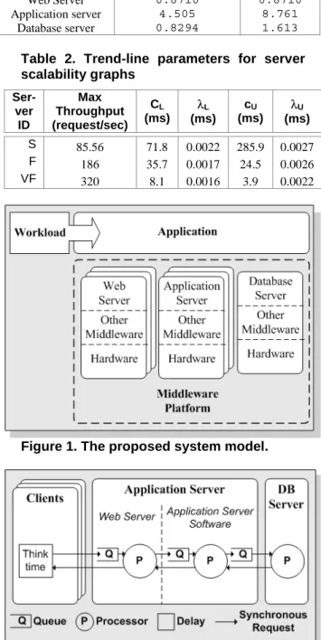
3. e-Commerce System Model

This section details a common architecture for e-Commerce applications. This architecture is derived in part from a case study of IBM Websphere [6]; a commercial platform for Java 2 Enterprise Edition (J2EE) applications. In the architecture (see figure 1), applications run on a middleware platform broken down into: the processing on one of a choice of web servers (for returning static web pages), the processing on one of a choice of application servers; and the data access on a single database server. Such platforms are typically multi-layered so these servers can run on other layers including Java virtual machines and the operating system. Each layer provides some of the functionality that applications require, which can dramatically increase software complexity [7]. The workload is broken down into ‘request types’ that are expected to exhibit similar performance characteristics due to the operations being called and the amount of data associated with the request.

Websphere includes a stock-trading benchmark known as ‘Trade’ with application server code designed to be representative of industrial strength J2EE e-Commerce applications [8]. Trade (v2.5.1) and the Websphere Application Server (v4.0.1) are used as a case study. Although alternative e-Commerce benchmarks with more sophisticated multi-server architectures exist (i.e. TPC-W [9]), the focus of this study is on the performance of the application server.

Performance models of this kind of system must be able to predict QoS metrics on heterogeneous servers and handle the fact that the performance of both the application and platform can vary dynamically. For example, application performance could vary due to functionality or content changes, and platform performance could change due to configuration updates. It can also be advantageous to: model the performance of the system at a coarse granularity (such as the application server level) due to monitoring overheads; and to rely on a definition of a ‘typical’ application-specific workload (which may be dynamically updated) so as to be able to quickly benchmark new servers. This is in contrast to the PACE approach, which involves creating separate models of the application and resource using static fine-granularity modelling.

This paper focuses on modelling the effect on response times and throughputs of allocating workload to heterogeneous application servers in dynamic e-Commerce systems. The main resource demand considered is CPU demand, as application servers in production environments are often connected by a high speed LAN to minimise network delay, and have sufficient RAM so as to minimise disk demand [10]. These assumptions can be verified via monitoring.

4. Queuing Network Modelling

This section discusses applying layered queuing modelling to the e-Commerce system model described in the previous section. Layered queuing modelling is a technique that can identify key system performance parameters [11] and calculate the effects of queuing and competition between requests. Previous work on layered queuing modelling has involved applying it to a range of distributed systems [12,13], including e-Commerce systems (using the Trade/Websphere e-Commerce case study used in this paper) [10]. This paper extends that work, which focussed on static capacity sizing and quantifying the impact of the queuing network configuration, by comparing the ability of the modelling to make dynamic predictions on heterogeneous servers, with an alternative ‘historical data analysis’ approach.

A layered queuing model is created in which clients are assumed to only issue one request at a time, meaning requests (in effect) do not leave the system so a closed layered queuing model is used. In this context ‘client’ refers to a request generator (such as a web browser window) that requires the result of the previous request to send the next request. Users that start several such conversations can be represented as multiple ‘clients’. The sequence of requests/replies initiated by each request from a client is illustrated in figure 2. All requests are synchronous calls to the next server, during which the thread processing the request sleeps. Each server has one FIFO queue which is shared by all incoming requests. The processors in the client tier are considered to be infinite as the focus of this study is the application tier. Local communication delays can be incorporated as a fixed delay (for a particular data size).

The clients are assumed to have an exponentially distributed think-time between requests, which results in a Poisson distribution for the rate at which each client’s requests arrive at the application tier. The processing time at the application servers is assumed to be exponentially distributed.

The following are the system-wide parameters to the model:

• Workload: number of clients, the workload mix (the expected percentage of the different types of request received each second) and the mean client think-time.

• Queuing network configuration: the maximum number of requests each processor can process at the same time via time-sharing

variable to represent system load in this model. This is because it determines the average utilisation of the application server or, when this reaches maximum, determines the average size of the application server queue.

The following are the request type specific parameters:

• Application parameters: average number of database requests

• Platform parameters: mean processing times on each server (possibly calculated using an additional platform performance parameter: request processing ability under the ‘typical’ workload)

It is assumed that the current values of all the system parameters are known; for example they could be determined by monitoring changes to the incoming workload and system configuration. Unlike the system parameters, the request type specific parameters need to be calibrated.

Layered queuing models can also support heterogeneous client types, with different request mix and think-time parameters. In this case other metrics are used to represent system load, such as request arrival rate prior to max throughput being reached. External request arrivals are also supported (or they can be approximated as clients that only make one request).

Layered queuing networks can be solved using the associated PARASRVN simulator and LQNS analytical solver. These have been found to produce solutions after at least 10 minutes, and after a few seconds respectively, on a Pentium 4 1.8Ghz. This makes it impractical to use the simulator dynamically. The disadvantage of LQNS is that it is more likely to fail to converge or be inaccurate due to the assumptions made. However this was not found to be a problem in the experiments conducted.

4.1. Calibrating the Model

The per-request-type parameters are calibrated offline by sending a workload consisting only of that request type for an interval and monitoring the number of requests processed per second (i.e. the throughput) and the % CPU usage of each server. The number of database requests that a request type makes (nDB) from the application server is:

server n applicatio

server DB DB

throughput throughput n

_ _

=

The mean processing time for a request type on server

i (si) is calculated (in ms) as follows:

i i i

throughput used CPU

s

=

The next step is calibrating the model for ‘new’ servers that are homogeneous to the original with the exception of their platforms’ request processing speeds. To simplify the benchmarking of platform performance a ‘typical’ workload is defined. The benchmarking then involves sending a workload with the typical mix and think-time parameters at each server in turn, and the number of clients is increased until the max throughput is reached.

The difference between the servers’ request processing abilities is then defined as:

new orig

throughput mx

throughput mx

ratio throughput

_ _

_ = (3)

The processing times for the new server are defined as:

ratio throughput orig

s new

si( )= i( )× _ (4)

Other model parameters are unaffected by the change in the platform’s request processing speed.

An alternative to this approach would be to send the typical workload at a server at a small number of clients and calculate the mean processing time using equation 2. This could then be used to compare servers’ performances instead of a max throughput rating. This would require less workload generating capacity, but is yet to be applied in these experiments.

It will be necessary to occasionally recalibrate the platform specific parameters (i.e. by taking parts of the system offline) as variables that are not included as model parameters change. Examples include a change in platform performance due to logging or monitoring levels changing, or platform software upgrades. Recalibration could be initiated automatically by monitoring the accuracy of predictions to determine if the accuracy falls below a threshold.

4.2. Results

A layered queuing model of the Trade/Websphere case study will be used to generate ‘scalability’ graphs showing the predicted mean response times and throughputs of new heterogeneous application servers at different numbers of clients. Each application server will have its own web server running on the same machine.

A request type is created to represent the background load on the server (i.e. all workload other than the sample of client/s whose performance is being monitored). This background request type involves the next operation (buy/sell/quote etc…) being randomly selected, with probabilities defined as part of the Trade benchmark as being representative of real e-Commerce clients. The mean client think-time is 7 seconds.

request type is defined for modelling the (single) client that samples the response times of the buy operation with a think-time of 0 seconds. A ‘register new user’ request is also sent every 10 requests (but not sampled) since the data returned by a buy request includes a list of the stocks in the client’s portfolio. The request type therefore represents a workload with a mean portfolio size of 5.5.

Trade is calibrated on a ‘fast’ server AppServF (P4

1.8Ghz, 256MB heap) as detailed in table 1. It is found that buy requests take approximately twice as much CPU time as background workload requests. Buy requests make 2 database requests, and background requests make 1.14 database requests on average. Due to the implementation of the Trade application all requests are for dynamic content, so the web server just makes a synchronous call to the application server for each request. As a result, queuing network configuration parameters are set so the maximum number of requests that can be processed at the same time is 50 for both application servers and 20 for the database server.

The next step is to determine the max throughputs on AppServF, a new ‘slow’ server AppServS (P3 450Mhz,

128MB heap) and a new ‘very fast’ server AppServVF,

(P4 2.66Ghz, 256MB heap), under the background request type. The heap size is smaller on the slow server due to limited memory on the machine, but is found to be adequate. The maximum throughputs are found to be 186, 86 and 320 requests/second respectively, allowing the new servers to be calibrated as described previously.

The background request type is generated on up to 12 PCs, each of which simulate 250 clients using Apache JMeter 1.8 [14]. An additional instrumented workload is run on a separate machine using an in-house Java program to sample response times of the buy request type. On AppServVF the client is run on the server so as to have the same system clock as the response time breakdown sensors. A minimum of 100 samples per graph data point are measured. The client machines (P4 1.8Ghz, 512MB RAM) run on Red Hat Linux 9, the database (DB2 7.2 on an Athlon 1.4Ghz, 512MB RAM) and application servers (using IBM HTTP Server 1.3.19 as the web server) run on Windows 2000 Advanced Server.

Figure 3 shows the response time breakdown for AppServVF. This graph shows how as maximum

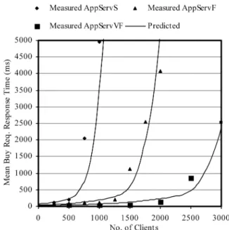
throughput is reached the queuing component of the response time becomes most significant (due to the queue being on average non-empty). Below 2000 clients the database component of the response time is most significant. However the performance of the database is constant for the heterogeneous application servers due to it being lightly loaded and application servers being tested separately. Figures 4 and 5 show the predictions for throughput and mean response time.

Figure 4 shows how application server throughput increases linearly as the number of clients is increased

until maximum throughput is reached. The point at which this levelling off happens normally corresponds to the % CPU utilisation metric reaching 100%, assuming there are no bottlenecks such as an insufficient number of application server threads. A minor inaccuracy is that since the connection overhead is not modelled the predicted throughputs become less accurate after max throughput is reached.

Figure 5 shows how the mean response time metric increases exponentially with the number of clients. Prior to maximum throughput being reached, the increase in response time is due to the increase in the average number of requests being processed at once. As maximum throughput is approached the increase in response time changes so as to become due to the increase in the average size of the queue. As maximum throughput is reached a significant discontinuity in the rate at which response times increase can be observed; an important behaviour for workload managers to be aware of.

It is also observed that the response times tend to be slightly less for measurements taken later in each sample. This suggests that the real queuing network might not have been reaching a steady state, whereas the LQNS solver that was used can only make predictions for the steady state. However the shapes of the graphs are predicted accurately, and the mean accuracy of the predictions for the established server is 2.2% for throughput, and 28% for mean response time; the mean accuracy for the new servers is 2.9% for throughput, and 37% for mean response time.

5. Historical Data-based Modelling

This section discusses applying an alternative modelling approach (historical data analysis-based performance modelling) to the e-Commerce system model described in section 3. Previous work on the historical data analysis approach includes an investigation into the metrics that can be used to represent e-Commerce system loads [15]. Other work includes an approach for evaluating the accuracy of predictions [16,17].

The historical approach involves sampling and recording request response times as the e-Commerce system runs. Response times are recorded in a historical performance repository along with other variables representing the workload being processed and platform performance information, at the time. For this experiment only the following variables, as also modelled in section 4, are recorded:

• the number of clients connected to the application server

The modelling process involves determining the relationship between each variable and request response times as discussed in the rest of this section. The relationships for other variables could be determined in a similar fashion. For example it is likely that load-independent weights could be associated with the different request types to define their relative resource demands. Heterogeneous workload could then be accounted for by introducing the mean request mix ‘weight’ of a client-type as an additional variable. As an alternative to modelling every variable, ‘old’ measurements could be phased out of the repository to increase predictive accuracy, for example if a platform’s performance changes due to monitoring or logging settings being changed.

5.1. Results

This section presents results showing how mean response time and throughput scalability graphs for proposed servers can be estimated based on the scalability graphs of established servers. As discussed in the queuing network section, the number of clients can be used as the main variable for system load given the assumptions made. There is a linear relationship between the number of clients and throughput, until the max throughput for the server under that particular workload is reached. Before max throughput is reached this has the form:

clients no

m

throughput= × _ (5)

where m is calculated from the historical data. After max throughput is reached the throughput is assumed to be roughly constant. It is straightforward to use this relationship to generate predicted throughput scalability graphs for servers with heterogeneous CPU speeds since the value of m appears to be constant across different CPU speeds (0.14 for all servers in the experimental setup). When applied to the measured data in figure 4, this gave a prediction accuracy of 1.3%.

When the client think-time is non-zero there is an exponential relationship between number of clients and mean request response time. However there is a discontinuity in this exponential relationship around the point that max throughput is reached. This results in two exponential scalability lines:

clients of no Le L

c

mrt= λ* _ _ (6)

clients of no Ue U

c

mrt= λ * _ _ (7)

for before and after max throughput is reached, respectively, where mrt is the mean response time and cL,

cU, λL and λU are calculated from historical data (although

in practice we have found that making the change from equation 6 to equation 7 shortly before max throughput is reached, and allowing for some overlap can increase

predictive accuracy). To investigate this, the scalability graph for a ‘new’ server (AppServVF) will be extrapolated

from the scalability graphs for two established servers (AppServS and AppServF). The parameters for cL, cU, λL

and λU for the three scalability graphs for these servers

are calculated (from lines of best fit for the measured data in figure 5) as shown in table 2. It is assumed that the max throughputs of all three servers, and the scalability graphs parameters for the two established servers, are known.

We have found that the following functions approximate the relationship between the max throughput of an application server and the parameters c and λ in its scalability graph, in our experimental setup:

) ( _

)

( cL

L

L C c mx throughput

c = × ∆ (8)

throughput mx

L

L C e L

_ )* ( )

(λ λ

λ _{= ×} ∆ ₍₉₎

) (

_ )

( cU

U

U C c mx throughput

c = × ∆ (10)

throughput mx

U

U C e U

_ )* (

) (λ λ

λ _{= ×} ∆ ₍₁₁₎

Values were then found for the C and Λ parameters by fitting lines of best fit to the two established servers, resulting in ‘lower’ and ‘upper’ equations for mean response time, from equations 6 and 7. A third equation is then defined for a ‘transition’ interval for when:

2 _

_clients no clients z

no ≥ _MT − (12)

and:

2 _

_clients no clients z

no ≤ _MT + (13)

where no_clientsMT is the number of clients at which

max throughput is reached, and z is the size of the interval (set at 500 clients in the experimental setup). When the number of clients is within this interval the equation for mean response time is:

clients of no L Lc e L

W

mrt= λ× _ _

clients of no U Uc e U

W × _ _

+ λ (14)

where:

+ =0.5

U W z clients no clients

no_ _ _MT)

( −

(15)

and:

U

L W

W =1− (16)

samples per graph data point. The predictive accuracy is likely to improve given data from additional heterogeneous servers, and by refining the variable relationships used to make predictions.

The runtime operation of the historical extrapolation service (and how monitoring granularity and sampling rate are tuned to balance overheads, predictive accuracy and the speed at which predictions are made) will be the subject of a future paper.

6. Discussion

The two approaches are compared as follows (where reference to ‘layered queuing’ refers not to the modelling technique in general, but to the specific modelling approach proposed in this paper):

• Creating the model: there is more flexibility for the historical modelling to be done at runtime, than with the layered queuing approach. This would allow relationships between variables to take into account factors such as unforeseen bottlenecks, and for requests to be grouped into request types with similar performance based on the actual, as opposed to expected workload.

• Collecting data: the overhead of the comprehensive monitoring in the historical approach is likely to be significantly greater than the predictive accuracy monitoring and recalibrations in the layered queuing approach.

• Evaluating the model at runtime: The accuracy of historical models increase with the number of variables considered, the amount of data available for each variable and how spread out the data is across the potential range of values (which could involve the number of heterogeneous servers being a limiting factor). The layered queuing approach is not limited by a shortage of data assuming model parameters are known, but does require the solver to converge.

• Adaptiveness: The historical approach is much more flexible in how it can cope with unexpected changes to the workload and platform performance. Examples include turning on additional monitoring or phasing out old data from the repository. The layered queuing approach is more restricted in that its main response is to re-calibrate a model.

Overall the historical approach has a higher monitoring overhead but has the potential to be more adaptive at runtime, taking into account unforeseen workloads, platform performance changes and bottlenecks. This is likely to increase accuracy (or reduce overheads) but at the cost of more complex runtime operation. However, although the layered queuing approach is more limited in how it can take into account unmodelled performance

variations and requires the ability to generate a representative workload, it is potentially simpler and gives a parameterised model that can be evaluated quickly.

The decision as to which approach is best for a particular system will involve finding a balance between model creation and monitoring costs and the expected accuracy of predictions over the lifetime of the system. For example the more limited costs in the layered queuing approach may make it the most appropriate choice for many systems (assuming system performance has been tuned to avoid bottlenecks). However the historical approach is likely to be more appropriate for the creation of adaptive models for more accurate predictions over the lifetime of highly dynamic systems. Applying both approaches together (for example refining layered queuing predictions using historical data) could also, despite the potential increase in model complexity, help achieve a good balance and is a topic that will be investigated in future work.

7. Conclusions

This paper reports on how two performance modelling approaches (based on layered queuing modelling and historical data analysis) are being applied to the performance prediction of dynamic e-Commerce applications running on heterogeneous servers. Results are presented showing how the response time and throughput versus number of clients scalability graphs, that will be provided by an e-Commerce benchmark on proposed servers with varying processing speeds, can be predicted using both approaches. The approaches are compared and their usefulness to Grid workload managers is considered. Future work will include predicting QoS metrics based on response time variances and deadlines, and investigating how this work might be used to also predict the cost of workload re-allocations so as to integrate with dynamic server allocation policies [18].

Acknowledgments

References

[1] I. Foster, C. Kesselman, J. Nick, S. Tuecke, “Grid Services for Distributed Systems Integration”, IEEE Computer, 35(6):37-46, 2002

[2] G. Nudd, D. Kerbyson, E. Papaefstathiou, S. Perry, J. Harper and D. Wilcox. “PACE: A toolset for the performance prediction of parallel and distributed systems”, International Journal of High Performance Computing Applications, 14(3):228–251, 2000

[3] J. Cao, D. Kerbyson, E. Papaefstathiou, and G. Nudd. “Performance modelling of parallel and distributed computing using PACE”, 19th IEEE International Performance, Computing and Communication Conference, pp 485–492, 2000

[4] S. Perry, R. Grimwood, D. Kerbyson, E. Papaefstathiou, and G. Nudd. “Performance optimisation of financial option calculations” Parallel Computing, 26(5):623–639, 2000. [5] A. Alkindi, D. Kerbyson, and G. Nudd. “Optimisation of

application execution on dynamic systems” Future Generation Computer Systems, 17(8):941–949, 2001

[6] M. Endrel, IBM WebSphere V4.0 Advanced Edition Handbook, IBM International Technical Support Organisation Pub., 2002. Available at: http://www.redbooks.ibm.com/

[7] R. Berry, “Trends, Challenges and Opportunities for Performance Engineering with Modern Business Software”, IEE Proceedings-Software Special Issue on Performance Engineering, 150(4), 2003

[8] IBM Websphere Performance Sample: Trade2. Available at http://www.ibm.com/software/

webservers/appserv/wpbs_download.html

[9] Transaction Processing Performance Council, “TPC-W Specification v1.8”, February 2002, Available at: http://www.tpc.org/tpcw/

[10] T. Liu, S. Kumaran, and J. Chung, “Performance Modeling of EJBs”, SCI2003 7th World Multiconference on Systemics, Cybernetics and Informatics, Florida USA, 2003

[11] John Dilley, Tai Jin, Richard Friedrich, Jerome Rolia, “Web Server Performance Measurement and Modeling Techniques”, Performance Evaluation, 33:5-26, 1998. [12] C.M. Woodside, J.E. Neilson, D.C. Petriu, S. Majumdar,

“The Stochastic Rendezvous Network Model for Performance of Synchronous Client-Server-like Distributed Software”, IEEE Trans. On Computer, 44(1):20-34, 1995. [13] M. Woodside, “Software Performance Evaluation by

Models”, Performance Evaluation, LNCS 1769, pp. 283-304, 2000.

[14] Apache JMeter User Manual. Available at: http://jakarta.apache.org/jmeter/index.html

[15] D.A. Bacigalupo, J.D. Turner, S.A. Jarvis, and G.R. Nudd, “A Dynamic Performance Prediction Framework for e-Commerce Applications”, Invited Paper at SCI2003 7th World Multiconference on Systemics, Cybernetics and Informatics, Florida USA, 2003, pp 390-395

[16] J.D. Turner, D.P. Spooner, J. Cao, S.A. Jarvis, D.N. Dillenberger and G.R. Nudd, “A Transaction Definition Language for Application Response Measurement” International Journal of Computer Resource Measurement, 105:55-65, 2001

[17] J.D. Turner, D.A. Bacigalupo, S.A. Jarvis, D.N. Dillenberger and G.R. Nudd, “Application Response Measurement of Distributed Web Services”, International Journal of Computer Resource Measurement, 108:45-55, 2002

[18] J. Palmer, I. Mitrani, “Dynamic Server Allocation in Heterogeneous Clusters”, Technical Report CS-TR:799, School of Computing Science, University of Newcastle, 2003

Table 1. AppServF mean processing times

Processor Background (ms) Buy (ms)

Web Server 0.8710 0.8710

Application server 4.505 8.761

Database server 0.8294 1.613

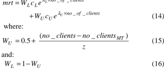
Table 2. Trend-line parameters for server scalability graphs

Ser-ver ID

Max Throughput (request/sec)

CL

(ms) λ

L

(ms) cU

(ms) λ

U

(ms)

S _{85.56 71.8 0.0022 285.9 0.0027} F _{186 35.7 0.0017 24.5 0.0026} VF _{320 8.1 0.0016 3.9 0.0022}

Figure 1. The proposed system model.

Figure 3. Response time breakdown for AppServVF showing the queuing and

processing components of the overall response time at the application and database servers.

Figure 4. Predicting the throughput scalability graphs for two new servers (AppServS and AppServVF), based on a

queuing model calibrated on an established server (AppServF). Linear trendlines are

shown for the predicted throughputs.

Figure 5. Predicting the response time scalability graphs for 2 new servers (AppServS and AppServVF), based on a

queuing model calibrated on an established server (AppServF).

Figure 6. Predicting the scalability graph for a new server (AppServVF), based on historical data

from 2 established servers. To enhance graph clarity additional AppServS measured response