Research on the Relationship between CPI and PPI Based on VEC Model

(1)

http://www.scirp.org/journal/ojs ISSN Online: 2161-7198

ISSN Print: 2161-718X

DOI: 10.4236/ojs.2019.92016 Apr. 12, 2019 218 Open Journal of Statistics

Research on the Relationship between CPI and

PPI Based on VEC Model

Shijun Li, Guoqiang Tang

*

, Duancui Yang

*

, Shixue Du

School of Science, Guilin University of Technology, Guilin, China

Abstract

By establishing the VEC model, the relationship between Consumer Price Index (CPI) and Producer Price Index (PPI) is explored by using Johansen cointegration test and impulse response function. The results show that there is a long-term equilibrium cointegration relationship between CPI and PPI. CPI has a certain impact on PPI. PPI also has a certain impact on CPI. PPI has a great impact on itself both in the long-term and short-term. The current CPI will be adversely affected by the previous CPI and the positive impact of the previous PPI. The current PPI will be positively affected by the previous phase of CPI and the previous phase of PPI.

Keywords

VEC Model, Consumer Price Index, Producer Price Index, Impulse Response Function

1. Introduction

The degree of inflation is mainly measured by the price index. The most impor-tant indicator is the Consumer Price Index (CPI), and Producer Price Index (PPI) can help determine the status quo and trends of inflation. CPI mainly re-flects the price changes of daily life commodities and service items of urban households. It is one of the important indexes for judging the degree and trend of inflation. CPI is divided into food, tobacco, alcohol and supplies, household equipment and maintenance services, health care and personal goods, transpor-tation and communications, entertainment, education, cultural goods and ser-vices, and housing. PPI can be regarded as the most important price index of the mid-stream industry, and it plays a role in the product price trend. PPI represents the production materials and consumer goods sold by industrial en-terprises to commercial, foreign trade, materials, residents or other industries

How to cite this paper: Li, S.J., Tang, G.Q., Yang, D.C. and Du, S.X. (2019) Research on the Relationship between CPI and PPI Based on VEC Model. Open Journal of Statistics, 9, 218-229.

https://doi.org/10.4236/ojs.2019.92016

Received: March 14, 2019 Accepted: April 9, 2019 Published: April 12, 2019

(2)

DOI: 10.4236/ojs.2019.92016 219 Open Journal of Statistics

and sectors. It reflects the impact of ex-factory price changes on industrial out-put value within a certain period of time. It is not only the main indicator for judging inflation, but also the important basis for the formulation of policies PPI covers more than 4000 products in 39 industrial sectors. The National Bureau of Statistics divides the PPI into production data PPI and living data PPI. The pro-duction data PPI can be subdivided into extractive industry propro-duction data PPI, raw material production data PPI and processing industry production data PPI. And living data PPI can be subdivided into food products PPI, clothing PPI, general merchandise PPI and consumer durables PPI. Economic life can be un-derstood depth by studying the relationship between CPI and PPI [1].

Through the price conduction law, the fluctuation of PPI will be transmitted to CPI. In turn, the fluctuation of CPI will also affect PPI. The two price indices can be described as an industrial chain connecting from upstream production to downstream consumption. PPI reflects upstream. With changes in production prices, CPI reflects changes in downstream consumption. According to the theory of production chain transfer, from the perspective of supply shock, price fluctuations are generally transmitted from upstream to downstream. Eventual-ly, the fluctuation of PPI will cause CPI changes, but there will be a certain lag period; demand decision theory holds that the ultimate goal of all economic ac-tivities is to provide goods and services to consumers, so the consumer’s demand will determine the price of these final consumer goods, and ultimately reflect the reverse mechanism of CPI to PPI. More research shows that the causal relation-ship between CPI and PPI is not one-way, but two-way, complex and non-linear

[2]. The difference in CPI-PPI reflects the growth of corporate earnings: CPI-PPI has a strong leading role in industrial enterprise profits. The CPI-PPI indicator also has a strong correlation with the overall growth rate of the economy. The smaller the difference of CPI-PPI, the higher the operating cost of the enterprise, the lower the profit of the enterprise, the slower growth of the profit of the en-terprise, and the slower economic growth. The greater the difference between CPI and PPI, the more the corporate profits are rebounding. The growth rate of cor-porate profits is rising, and the economic growth momentum is strong.

(3)

Previous studies have shown that there is a certain relationship between CPI and PPI, and both are important indexes reflecting the trend of economic de-velopment. Therefore, this paper studies the relationship between CPI and PPI by fitting the VEC model, and in-depth study of its internal relationship will help to understand the internal law of macroeconomic operation and facilitate the formulation and implementation of policies. The structure of the article is as follows: Section 1 is the introduction; Section 2 is the model introduction and modeling steps; Section 3 is the empirical study; Section 4 is the conclusion.

2. Model Introduction and Modeling Steps

2.1. VAR Model

The vector autoregressive model (VAR model) was proposed by Sims C A in 1980 and is mainly used to analyze and predict the dynamic impact of random disturbance on the system, the magnitude of the impact, the positive and nega-tive and the duration of time [8]. The focus of the VAR model is not on inter-preting the estimated parameters, but on interinter-preting and analyzing the interre-lationships among the variables through the impulse response function and the variance decomposition.

Let Yt =

(

y1t,y2t,,ynt

)

′ denote an (n × 1) vector of time series variables.

The basic p-lag vector autoregressive (VAR(p)) model has the form:

1 1 2 2 , 1, 2, ,

t t t p t p t

Y = + ∏c y− + ∏ y− + + ∏ y− +ε t= T (1)

where ∏i are (n n× ) coefficient matrices and εt is an (n × 1) unobservable

zero mean white noise vector process (serially uncorrelated or independent) with time invariant covariance matrix ∑. The stability condition of the VAR(p) model is that the characteristic equation is required. ∏ − Ε =i λ 0 The roots are

all within the unit circle.

2.2. Johansen Cointegration Test [9]

In 1990, Johansen and Juselius proposed the Johansen cointegration test, which is a test method for testing regression coefficients based on the VAR model, and can also be used for cointegration tests between multiple variables.

For

(

1, 2, ,

)

T

t t t nt

Y = y y  y , a cointegration definition can be used to discuss whether there is a cointegration relationship between this variable. The defini-tion of cointegradefini-tion is as follows:

The components of the n-dimensional vector time series Yt are called d, b-order cointegration. Recorded as Yt ~CI d b

( )

, , if the following two points are

met:

1) Yt ~I d

( )

, require that each component of Yt is d-order and monolithic;

2) There is a non-zero vector β, make β ′Yt ~I d

(

−b

)

, 0< ≤b d.

The abbreviation Yt is cointegration, and the vector β becomes a

cointe-gration vector.

There are at most n − 1 linearly independent cointegration vectors for the

(4)

2.3. The Basic Idea of Impulse Response Function [10]

In practical applications, because the VAR model is a non-theoretical model, it does not have to make any a priori constraints on the variables, so when analyz-ing the VAR model, it is generally not analyzed that one variable will produce another variable. How to influence, but to analyze the dynamic impact on the system when an error term changes, that is, when the model is subjected to some kind of impact, this analysis method is called the impulse response function.

The impulse response function analysis method can be used to describe the response of the impact of the error term on the endogenous variable, that is, the impact of the impact of one standard deviation on the random error term on the current value and future value of the endogenous variable.

The basic idea of the impulse response function analysis method is introduced below by taking the VAR(2) model with two variables as an example.

1 1 1 1 2 1 2 1 2 1 2 2 2 1

2 1 1 1 2 1 2 1 2 1 2 2 2 2

, 1, 2, ,

t t t t t t

y a y a y b y b y

t T

y c y c y d y d y

ε ε − − − − − − − − = + + + +  =  ₌ ₊ ₊ ₊ ₊

  (2)

In formula (2), Pending parameter a b c di, , ,i i i, εt =

(

ε ε1t, 2t

)

′ random

dis-turbance. Assume that it is a white noise vector with the following properties:

( )

(

)

(

)

0, , 1, 2

var { },

0, , 1, 2 it

t t t ij

it is t i

t

t s i

ε

ε ε ε σ

ε ε

Ε = ∀ = ′

= Ε = ∑ = ∀ Ε = ∀ ≠ =

(3)

Assume that it is starting from the 0th period, and set

1 1t 1t 2 2t 1 2t 2 0

y − = y − =y − = y − = ,

Also set in the 0th period given the disturbance term ε =10 1, ε =20 0, And

other disturbance items are 0. ε1t =ε2t=0

(

t=1, 2,

)

. This is called the

im-pulse response of phase 0 to y1t.

2.4. VEC Model [10]

Engle and Granger combine the cointegration theory with the error correction model to establish a vector error correction model, the VEC model. As long as there is a cointegration relationship between the variables, the error correction model (ECM) can be derived from the autoregressive distribution lag model. In the VAR model, each equation is an autoregressive distribution lag model. Therefore, we can think that the VEC model is a VAR model with cointegration constraints.

According to the cointegration equation, the expression of the VEC model can be obtained:

1

1 1 p

t t i t i t

i

y αβ y y µ

−

− −

=

′

∆ = +

∑

Γ ∆ + ₍₄₎

among them,

1 p

i j

j i= +

Γ = −

∑

∏ _, ∆y_t is the stationary value of yt after differential

transformation,

α

is a coefficient vector, β is a cointegration vector, and µt

(5)

Equation (4) can also be expressed as:

1

1 1 ecm

p

t t i t i t

i

y α y µ

−

− −

=

∆ = ⋅ +

∑

Γ ∆ + (5)

Each equation in Equation (5) is an error correction model. Where

1 1

ecmt− =β′yt− is the error correction term vector, reflecting the long-term

equilibrium relationship between variables. The coefficient vector

α

_reflects

the adjustment speed of the variable to the equilibrium state when it deviates from the long-term equilibrium state. All coefficients of the difference term as explanatory variables reflect the effect of short-term fluctuations of each variable on short-term changes as explanatory variables.

2.5. Modeling Steps

This paper explores the relationship between CPI and PPI by establishing a VEC model and using co-integration test and impulse response function. The model-ing steps are as follows:

1) In order to eliminate seasonal trends and heteroscedasticity and reduce fluctuations, first-order differences between CPI sequences and PPI sequences to conduct DCPI and DPPI sequences;

2) Perform unit root test on sequence CPI, PPI, DCPI, DPPI;

3) Determining the maximum lag order p of the VAR model by the SC criterion; 4) Construct the VAR(p) model with the maximum lag order p, and verify the stability of the VAR(p) model using the AR root chart;

5) Johansen cointegration test on the first-order single-sequence CPI and PPI, and check whether there is a long-term cointegration relationship;

6) Based on the cointegration test, the impulse response function of the VAR model is analyzed;

7) Explore the short-term fluctuations and long-term equilibrium between CPI and PPI through the VEC model.

3. Empirical Research

3.1. Data Source

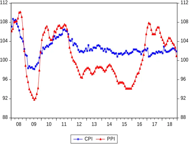
The data in this paper comes from the Eastern Fortune Network. The monthly data of China’s consumer price index (CPI) and industrial producers’ price in-dex (PPI) from January 2008 to December 2018 are selected. The total data are 132 months. Figure 1 shows time series chart of the Consumer Price Index (CPI) and the Producer Price Index (PPI). It can be seen from Figure 1 that the PPI is always higher than CPI from November 2016 to November 2018. PPI fluctuates sharply compared to CPI.

3.2. Sequence Stability Test

(6)

[image:6.595.216.533.75.316.2]

Figure 1. Time series diagram of CPI and PPI.

obviously stronger than that CPI sequence. From the objective point of view, it is necessary to judge the stationarity of the sequence by unit root test. In order to eliminate seasonal trends and heteroscedasticity and reduce fluctuations, the se-quence CPI and PPI are subjected to first-order difference respectively, and the generated sequences are recorded as sequence DCPI and DPPI respectively, and the unit root test are performed on the two sequences. The P-value is defined as the probability, under the null hypothesis H, Pr

(

X ≥x H

)

for right tail event,

(

)

Pr X ≤x H for left tail event, 2 min Pr

{

(

X ≤x H

) (

, Pr X ≥x H

)

}

for double tail event.

It can be seen from Table 1 that the ADF test values of the sequence CPI and PPI are greater than the t-statistic thresholds of the test levels of 1%, 5%, and 10%, and the probability P values are all greater than 0.10. The original hypothe-sis cannot be rejected, the sequence CPI and PPI are non-stationary sequence. The differenced sequence is DCPI and DPPI. The ADF test value is less than the

t-statistic threshold of 1%, 5% and 10% of the test level, and the probability P

value is less than 0.01, which means the sequence DCPI and DPPI are considered to be stationary sequences. The sequence CPI and PPI are first order single-order se-quences, indicating that the two may have a long-term co-integration relation-ship.

3.3. VAR Model Maximum Lag Order

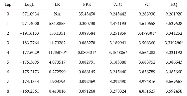
Before constructing the VAR model, the Schwartz Criterion (SC) was used to determine the maximum lag order p of the model. The results are shown in Ta-ble 2.

It can be seen from Table 2 that the minimum of order P corresponding to

88 92 96 100 104 108 112

08 09 10 11 12 13 14 15 16 17 18

(7)

[image:7.595.210.539.91.192.2]

Table 1. Unit root test results of two sequences.

sequence ADF test value Significant level P value Stationarity

1% 5% 10%

CPI 0.066846 −2.584539 −1.943540 −1.614941 0.7022 Non-stable PPI −0.707841 −2.583011 −1.943324 −1.615075 0.4084 Non-stable DCPI −6.427866 −2.584539 −1.943540 −1.614941 0.0000 smooth DPPI −4.920177 −2.583011 −1.943324 −1.615075 0.0000 smooth

Table 2. Maximum lag order selection criteria.

Lag LogL LR FPE AIC SC HQ

0 −571.0934 NA 35.43458 9.243442 9.288930 9.261920 1 −271.4000 584.8855 0.300730 4.474193 4.610658 4.529628 2 −191.6153 153.1351 0.088584 3.251859 3.479301* 3.344252 3 −183.7764 14.79282 0.083278 3.189941 3.508360 3.319290* 4 −177.6029 11.45070* 0.080431* 3.154886* 3.564282 3.321192 5 −175.3695 4.070517 0.082791 3.183380 3.683752 3.386643 6 −175.2173 0.272599 0.088145 3.245440 3.836789 3.485660 7 −174.1344 1.903796 0.092469 3.292490 3.974816 3.569667 8 −169.2561 8.419016 0.091268 3.278324 4.051627 3.592458

the SC is 2, so the VAR model selects the lag order P = 2 as the maximum lag order.

3.4. Establishment and Verification of VAR Model

To establish a matrix form of the VAR(2) model:

1

2 2 CPI 8.916056 0.768439 0.219738 CPI PPI 3.592720 0.180074 1.743875 PPI

0.138832 0.214378 CPI 0.169544 0.790326 PPI

t t

t

t t

µ µ

−

      

= +

      

      

−  

  

+_ _ _ _{+ } _

− −

    

(6)

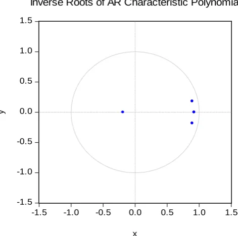
The SC value of the VAR(2) model is 3.479301, and the SC value is the smal-lest, indicating that the established VAR(2) model works well. In order to verify the smoothness of the VAR model, the AR root chart is used for verification. It can be seen from Figure 2 that the modulus of all unit root reciprocals falls within the unit circle, which means the established VAR(2) model is stable. The

X and Y axes of Figure 2 represent the coefficients of the eigenvalues, respec-tively. The four points in the unit circle are (0.92, 0.00), (0.89, −0.18), (0.89, 0.18), (−0.19, 0.00).

3.5. Johansen Cointegration Test

[image:7.595.209.538.225.394.2]

(8)

[image:8.595.256.492.76.310.2]

Figure 2. Distribution of AR unit roots.

construction model. The purpose of the cointegration test is to test whether the causal relationship described by the regression equation is a pseudo-regression. That is to say, whether there is a long-term stable relationship between the va-riables. The cointegration test requires that each sequence must be a non-stationary sequence and single-order single-sequence. From the unit root test results, it can be known that the sequence CPI and PPI meet the requirements of the cointe-gration test.

It can be seen from Table 3 that at the 5% significance level, the trace statistic test value is greater than the critical value, and the p values of the first row and the second row are 0.0007 and 0.0025, both are less than 0.05, rejecting the null hypothesis that there’s no cointegration relationship. The conclusion is that there is a long-term cointegration relationship between the consumer price in-dex and the industrial producer’s ex-factory price inin-dex. After standardizing the cointegration coefficient, the resulting cointegration equation is as follows:

CPI=0.923276PPI+µt (7)

3.6. Analysis of Impulse Response Function

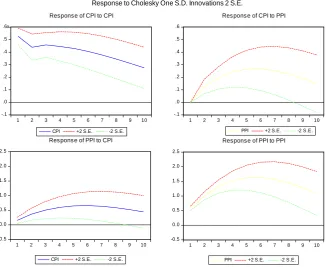
In order to describe the impact of a standard deviation on the random error term on the current and future values of the variable, this paper uses the impulse response function to analyze the response of consumer price index to the pro-ducer price index.

From the impulse response results in Figure 3, the impact of consumer price index on itself, reached a maximum of 0.53 at the first period, then began to de-cline to 0.44 of the second period, then rose to 0.46 in the third period, and then began a slow decline. It can be seen that consumer price index has short-term

-1.5 -1.0 -0.5 0.0 0.5 1.0 1.5

Inverse Roots of AR Characteristic Polynomia

y

(9)

[image:9.595.210.539.90.151.2]

Table 3. Johansen cointegration test results.

Null hypothesis:

[image:9.595.212.539.167.434.2]

Number of cointegration vectors Eigenvalues Trace statistics 0.05 significance level P value None* 0.125653 26.57579 15.49471 0.0007 At most 1* 0.067747 9.119681 3.841466 0.0025

Figure 3. Synthesis of impulse response function.

interference to itself. In the long run, the impact of the consumer price index on itself cannot be ignored. Consumer price index did not respond immediately to the first phase of the producer price index, and began to rise with the extension of the lag period, the sixth period rose to the highest point of 0.27 and then gradually declined. Hence, whether in the long-term or short-term, although the consumer price index will have a certain impact on the producer price index, but the impact is not significant.

The producer price index began to respond to its own impact in the first phase, the fifth period reached a maximum of 1.63, and then began to decline but not to zero, indicating that the producer price index has a certain long-term impact on itself. The producer price index has a certain impact on consumer price index, in the sixth period, it reached a maximum of 0.66, and then began to slowly decline but not to zero.

To sum up: whether it is the impact of CPI on itself or the impact of PPI on CPI, and reversely, whether it is the impact of PPI on itself or the impact of CPI on PPI, it is always positive. However, this did not affect the long-term deviation between CPI and PPI under the new economic normal.

-.1 .0 .1 .2 .3 .4 .5 .6

1 2 3 4 5 6 7 8 9 10 CPI +2 S.E. -2 S.E. Response of CPI to CPI

-.1 .0 .1 .2 .3 .4 .5 .6

1 2 3 4 5 6 7 8 9 10 PPI +2 S.E. -2 S.E. Response of CPI to PPI

-0.5 0.0 0.5 1.0 1.5 2.0 2.5

1 2 3 4 5 6 7 8 9 10

CPI +2 S.E. -2 S.E. Response of PPI to CPI

-0.5 0.0 0.5 1.0 1.5 2.0 2.5

1 2 3 4 5 6 7 8 9 10

PPI +2 S.E. -2 S.E. Response of PPI to PPI Response to Cholesky One S.D. Innovations 2 S.E.

(10)

3.7. VEC Model Establishment and Parameter Estimation

According to Johansen’s cointegration test, there is a long-term cointegration relationship between the consumer price index and the producer price index. Based on the previous VAR(2) model, the VEC model can be established to ana-lyze the long-term stability relationship and short-term fluctuations between the two.

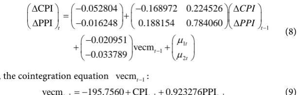
The VEC model is as follows:

1

1 1

2

CPI 0.052804 0.168972 0.224526 PPI 0.016248 0.188154 0.784060

0.020951 vecm 0.033789

t t

t

CPI PPI

µ µ

−

∆ − − ∆

      

= +

_∆  ₋   _∆ 

      

−  

 

+_ _ _{+ } _ −

   

(8)

where, the cointegration equation vecmt−1:

1 1 1

vecmt− = −195.7560 CPI+ t− +0.923276PPIt− (9)

[image:10.595.233.539.183.281.2]

From the estimation results of the VEC model, the SC value in the model is 1.711131, which indicates that the VEC model is very reasonable. It can be seen from the equation that CPI and PPI of the previous period have a positive effect on the current PPI. For each additional percentage-point increase in CPI of the previous period, the current PPI will increase by 0.188154 percentage-point; for each additional percentage-point increase in PPI of the previous period, the cur-rent PPI will increase by 0.784060 percentage-point. The CPI of previous period has a reverse effect on the current CPI, the PPI of previous period has a positive effect on the current CPI. For every one percentage-point increase in the pre-vious period of CPI, the current CPI will decrease by 0.168972 percentage-point; for each additional percentage-point increase in PPI of previous period, the cur-rent CPI will increase by 0.224526 percentage points. Vecm is an error correc-tion term, and its coefficient is negative, indicating that the CPI reversely corrects the CPI value of the next period with a value of 0.020951 to reach a long-term equi-librium state, and the PPI reversely corrects the PPI value of the next period with a value of 0.033789 to reach along-term equilibrium state.

Figure 4 is the cointegration curve between the CPI sequence and PPI se-quence. From 2008 to the end of 2011, the absolute value of the error correction term deviates greatly, especially in May 2008, August 2009, and August 2011. Short-term fluctuations deviate from long-term equilibrium. After 2012, the fluctuation range of the error correction item began to decrease, and gradually returned to the long-term equilibrium state, which was caused by a series of de-capacity, destocking, and supply-side reforms in China.

4. Conclusions

This paper uses the VEC model to empirically analyze consumer price index and producer price index, and studies the cointegration relationship between CPI and PPI, summarizing the following four points:

(11)

[image:11.595.233.515.73.268.2]

Figure 4. Cointegration diagram of CPI and PPI.

difference, and both belong to the first-order single-order sequence. Using the two-sequence lag phase 2 to be highly significant, the VAR(2) model was con-structed, indicating that the current consumer price index and the producer price index will be affected by the changes in the first two periods.

2) There is a cointegration relationship between CPI and PPI, which indicates that there is a long-term stable relationship between consumer price index and producer price index.

3) The impulse response of CPI and PPI indicates that CPI has long-term ef-fects on its own short-term fluctuations about whether it is from short-term fluctuations or long-term effects; CPI has certain impact on PPI, but the impact is not strong. PPI has a great impact on itself and has a long-term impact on CPI, but the impact is not big.

4) The VEC model analyzed the long-term stable relationship between CPI and PPI and the short-term fluctuations. The current CPI will be affected by the reverse impact of the previous CPI and the positive impact of the previous PPI. The current PPI will be affected by the previous CPI, the positive impact and the positive impact of the previous PPI. The coefficient error correction term is a negative value, which plays a role of inversely correcting the next period of CPI and PPI values to achieve a long-term equilibrium state.

Acknowledgements

Project supported by the National Natural Science Foundation of China (61703117); National Natural Science Foundation of China (61763008); Guangxi Young and Middle-aged Teachers’ Basic Ability Improvement Project (2018KY0261).

Conflicts of Interest

The authors declare no conflicts of interest regarding the publication of this paper. -15

-10 -5 0 5 10 15

08 09 10 11 12 13 14 15 16 17 18

(12)

References

[1] Hu, J.M. and Zeng, L.Q. (2017) Economic Stagflation Risk and Its Prevention.

Science Press, Beijing.

[2] Shi, K. (2016) Analysis of the VEC Model of CPI and PPI Relationship. Statistics

and Decision, No. 3, 83-86.

[3] Chen, Y. (2011) Research on the Relationship between PPI, Enterprise Commodity

Price Index, M2 and CPI. Journal of Liaoning University (Philosophy and Social

Sciences), 39, 97-103.

[4] He, L.P., Fan, G. and Hu, J.N. (2008) Consumer Price Index and Producer Price

In-dex: Who Drives Who? Economic Research, No. 11, 44-48.

[5] Xu, W.K. (2010) On the Consumer Price Index and Producer Price Index: Who

Drives Who? Questioning in a Paper. Economic Research, No. 5, 139-148.

[6] Yang, Z.H., Zhao, Y.L. and Liu, J.H. (2013) Nonlinear Study of CPI and PPI

Con-duction Mechanisms: Forward ConCon-duction or Reverse Thrust? Economic Research,

No. 3, 83-95.

[7] Yang, C. and Chen, L. (2013) Chinese CPI and PPI: Causality and Transmission

Mechanism. Journal of Xiamen University (Philosophy and Social Sciences), No. 3,

1-9.

[8] Sims, C.A. (1980) Macroeconomics and Reality. Econometrica,48, 1-48.

[9] Johansen, S. and Juselius, K. (1990) Maximum Likelihood Estimation and

Infe-rences on Cointegration—With Applications to the Demand for Money. Oxford

Bulletin of Economics and Statistics, 52, 169-210.

[10] Gao, T.M. (2016) Econometric Analysis Methods and Modeling—EViews