Topics in Tree-Based Methods

(1)

University of Pennsylvania

ScholarlyCommons

Publicly Accessible Penn Dissertations

1-1-2014

Topics in Tree-Based Methods

Alex Lauf Goldstein

University of Pennsylvania, [email protected]

Follow this and additional works at:http://repository.upenn.edu/edissertations Part of theStatistics and Probability Commons

This paper is posted at ScholarlyCommons.http://repository.upenn.edu/edissertations/1288

For more information, please [email protected].

Recommended Citation

Goldstein, Alex Lauf, "Topics in Tree-Based Methods" (2014).Publicly Accessible Penn Dissertations. 1288.

(2)

Topics in Tree-Based Methods

Abstract

This work introduces methods and associated software for enhancing the interpretability of fitted models, with emphasis on classification and regression trees. We begin in Chapter 1 by describing novel techniques for growing classification and regression trees designed to induce visually interpretable trees. This is achieved by penalizing splits that extend the subset of features used in a particular branch of the tree. After a brief motivation, we summarize existing methods and introduce new ones, providing illustrative examples throughout. Using a number of real classification and regression datasets, we find that these procedures can offer more interpretable fits than the CART methodology with very modest increases in out-of-sample loss.

These techniques are implemented in the R package itree, described in Chapter 2. In addition to the

procedures introduced in Chapter 1, itree implements a method for visualizing the out-of-sample risk as well as the usual classification and regression tree methodologies. Chapter 2 presents illustrative examples and demonstrates itree's usage for aspects of the software that are novel or unique to itree.

Whereas Chapters 1 and 2 relate to tree-based methods, Chapter 3 describes Individual Conditional Expectation (ICE) plots, a methodology for visualizing the model estimated by any supervised learning algorithm. Classical partial dependence plots (PDPs) help visualize the average partial relationship between the predicted response and one or more features. In the presence of substantial interaction effects, the partial response relationship can be heterogeneous. Thus, an average curve, such as the PDP, can obfuscate the complexity of the modeled relationship. Accordingly, ICE plots refine the partial dependence plot by graphing the functional relationship between the predicted response and the feature for individual observations. ICE plots highlight the variation in the fitted values across the range of a covariate, suggesting where and to what extent heterogeneities might exist. In addition to providing a plotting suite for exploratory analysis, we include a visual test for additive structure in the data generating model. The procedures outlined in Chapter 3 are available in the R package ICEbox.

Degree Type

Dissertation

Degree Name

Doctor of Philosophy (PhD)

Graduate Group

Statistics

First Advisor

Andreas Buja

Keywords

(3)

Subject Categories

(4)

TOPICS IN TREE-BASED METHODS

Alex L. Goldstein

A DISSERTATION

in

Statistics

For the Graduate Group in

Managerial Science and Applied Economics

Presented to the Faculties of the University of Pennsylvania

in

Partial Fulfillment of the Requirements for the

Degree of Doctor of Philosophy

2014

Supervisor of Dissertation

Signature Andreas Buja

The Liem Sioe Liong/First Pacific Company Professor of Statistics

Graduate Group Chairperson

Signature Eric Bradlow

Professor of Marketing, Statistics, and Education

Dissertation Committee

Richard A. Berk, Professor of Criminology and Statistics Ed George, Universal Furniture Professor of Statistics

(5)

TOPICS IN TREE-BASED METHODS

(6)

Dedication

(7)

Acknowledgments

(8)

ABSTRACT

TOPICS IN TREE-BASED METHODS

Alex L. Goldstein

Andreas Buja

This work introduces methods and associated software for enhancing the

inter-pretability of fitted models, with emphasis on classification and regression trees. We

begin in Chapter 1 by describing novel techniques for growing classification and

re-gression trees designed to induce visually interpretable trees. This is achieved by

penalizing splits that extend the subset of features used in a particular branch of

the tree. After a brief motivation, we summarize existing methods and introduce new

ones, providing illustrative examples throughout. Using a number of real classification

and regression datasets, we find that these procedures can offer more interpretable

fits than the CART methodology with very modest increases in out-of-sample loss.

These techniques are implemented in theRpackageitree, described in Chapter 2.

In addition to the procedures introduced in Chapter 1,itreeimplements a method for

visualizing the out-of-sample risk as well as the usual classification and regression tree

methodologies. Chapter 2 presents illustrative examples and demonstrates itree’s

usage for aspects of the software that are novel or unique to itree.

Whereas Chapters 1 and 2 relate to tree-based methods, Chapter 3 describes

Individual Conditional Expectation (ICE) plots, a methodology for visualizing the

model estimated byany supervised learning algorithm. Classical partial dependence plots (PDPs) help visualize the average partial relationship between the predicted

response and one or more features. In the presence of substantial interaction effects,

(9)

as the PDP, can obfuscate the complexity of the modeled relationship. Accordingly,

ICE plots refine the partial dependence plot by graphing the functional relationship

between the predicted response and the feature forindividual observations. ICE plots highlight the variation in the fitted values across the range of a covariate, suggesting

where and to what extent heterogeneities might exist. In addition to providing a

plotting suite for exploratory analysis, we include a visual test for additive structure

in the data generating model. The procedures outlined in Chapter 3 are available in

(10)

List of Tables

1.1 Summary of Notation . . . 4

2.1 Summary of Notation . . . 28

A.1 Scaling of Impurity Functions . . . 86

A.2 Defintions of One-Sided Impurity Functions . . . 87

A.3 OOB performance of penalization: CART on regression datasets . . . 89

A.4 OOB performance of penalization: One-Sided Purity on regression datasets . . . 90

A.5 OOB performance of penalization: High-Means on regression datasets 90 A.6 OOB performance of penalization: Low-Means on regression datasets 91 A.7 OOB performance of penalization: CART on classification datasets . 92 A.8 OOB performance of penalization: One-Sided Purity on classification datasets . . . 92

(13)

List of Figures

1.1 CART fit to the Boston Housing data . . . 7 1.2 CART fit to the Boston Housing data with and without the New

Vari-able Penalty . . . 12 1.3 CART fit to the Boston Housing data with the New Variable Penalty 13 1.4 One-sided High-Means fit to the Boston Housing data. . . 14 1.5 One-Sided Purity fit to the Pima data with and without the New

Vari-able Penalty . . . 15 1.6 CART fit to the Boston Housing data with the EMA-Style penalty . 17 1.7 High-Means fit to the Boston Housing data with the EMA penalty . . 17 1.8 One-Sided Extremes fit to the Pima data with and without the EMA

penalty . . . 18 1.9 One-Sided Purity fit to the Pima data with and without the EMA penalty 19 1.10 CART fit to the Red Wine data with and without the EMA Penalty . 22

2.1 CART and One-Sided Purity applied to the Boston Housing Data . . 31 2.2 CART and One-Sided Purtiy applied to the Pima Indians data . . . . 33 2.3 CART and One-Sided Purtiy applied to the Autism data . . . 34 2.4 Close-up: One-Sided Purity applied to the Autism data . . . 35 2.5 CART and One-Sided Purtiy applied to the Digit Recognition data . 36 2.6 CART and One-Sided Extremes applied to the Boston Housing data . 38 2.7 CART and One-Sided Extremes applied to the Digit Recognition data 39 2.8 Parsimony Example . . . 41 2.9 CART applied to the Boston Housing data with the New Variable Penalty 43 2.10 One-Sided Extremes applied to the Digit Recognition data with the

New Variable Penalty . . . 44 2.11 One-Sided Purity applied to the Pima Indians data with and without

(14)

3.1 Scatterplot and PDP of X2 versus Y for a sample from the process

described in Equation 3.3 . . . 58

3.2 SGB ICE plot for X2 from the data generating process described by Equation 3.3 . . . 59

3.3 RF ICE plot for the predictor agein the Boston Housing data . . . . 60

3.4 c-ICE plot for agewith x∗ set to the minimum value of age . . . 62

3.5 d-ICE plot for agein the BHD . . . 63

3.6 The c-ICE plot forage of Figure 3.4, colored by rm . . . 64

3.7 ICE and d-ICE plots for S =X1 for aGAM . . . 66

3.8 ICE plots for an SGBfit to the simple interaction model of Equation 3.6 68 3.9 ICE plots forS =x1 of aRF model fit to Equation 3.7 . . . 70

3.10 ICE plots of a BARTmodel for the effect of treatment on depression score 72 3.11 ICE plots of a NN model for wine ratings versus pH . . . 73

3.12 ICE plots for a RF for the variable skin coloredage . . . 75

(15)

1

Penalized Split Criteria for Interpretable Trees

∗

Abstract

This chapter describes techniques for growing classification and regression trees

de-signed to induce visually interpretable trees. This is achieved by penalizing splits

that extend the subset of features used in a particular branch of the tree. After a

brief motivation, we summarize existing methods and introduce new ones, providing

illustrative examples throughout. Using a number of real classification and

regres-sion datasets, we find that these procedures can offer more interpretable fits than the

CART methodology with very modest increases in out-of-sample loss.

1.1 Introduction

We assume familiarity with the techniques introduced in Breiman et al. (1984) for

fitting binary trees to data. For brevity we refer to these techniques both collectively

and individually by the acronym CART. Its authors state that CART is designed to

“produce an accurate classifier or to uncover the predictive structure” of a problem.

(16)

In comparison with the former task, the degree to which a model “uncovers structure”

eludes quantification. We offer no help on this front, but adopt Breiman et al. (1984)’s

preference for “simple characterizations of the conditions that determine when an

object is [in] one class rather than another” as our guiding principle, which we call

interpretability.

What is meant by a “simple characterization”? For classification trees, the question

of whether we predict yis in one class or another is determined by the terminal node

to which its associatedxvector belongs. Hence the conditions leading toy’s predicted

class are exactly the sequence of splitting rules that lead to its terminal node. As such,

the tree that offers the simpler sequence of splits also offers the simpler explanation of

y’s predicted class. In this sense, splitting procedures that encourage simple sequences

of split rules can result in particularly interpretable trees. Such procedures are the

focus of this chapter.

In Section 1.2 we review the fundamentals of CART, paying special attention to

gain and impurity, the critical functions for tree-growing. Further, we make the

no-tion of “simple sequences of splits” more precise. In Secno-tion 1.3 we present novel tree

growing techniques for the usual classification and regression settings where

inter-pretability is desirable. Section 1.4 reviews the out-of-sample performance of these

methods. The evidence suggests that in many cases the methods described in Section

1.3 yield interpretable trees with little sacrifice in generalization error. Section 1.5

(17)

1.2 Fundamentals of Classification and Regression

Trees

1.2.1 Splits and Splitting Criteria

Where possible we follow the terminology and notation of Breiman (1996b), as

out-lined below. Readers will recall that given a learning sampleLofN pairszi = (yi,xi)

from an arbitrary distribution in which _E(y|x) = f(x), the algorithms described in

Breiman et al. (1984) output a binary tree ˆf(x) that aims to approximatef or

thresh-oldf(x) whenyis binary. Here ˆf is called a classification or regression tree depending

on whether y is categorical or continuous, respectively.

For any x, ˆf(x) is given by the mean (for regression) or the most common (in

classification)yi value over alli∈ Lthat are in the same terminal node asx, denoted

byt(x). In either case, all observations in a given node tshare the same fitted value,

which we denote j(t) herein.

Each non-terminal node in the tree is defined by a splitting rule s. Each splitting rule comprises a pair (x, t) consisting of a variable x and a split location t. The rule

s= (x1,0), for instance, divides thentobservations intinto two subsets, depending on

whether eachxvector has a positive first coordinate. In this examplex1 is termed the

split variableand 0 thesplit point. Thegrowing phase consists of selecting the bestsat

tand then sendingt’s observations to the appropriate child nodes, where the recursion

begins anew. Though the details of both growing and pruning certainly influence

interpretability, our focus here is on tree-growing methods. Defining procedures for

choosing splits that lead to interpretable trees is the subject of Section 1.3.

(18)

at

s? = arg max s∈S

θ(t, s), (1.1)

meaning we choose the split that maximizes the split criterion, where S is the set of

all possible splits including no split. For CART,θ is of the form

θ(t, s) =φ(t)−

ntL nt

φ(tL) + ntR

nt

φ(tR)

, (1.2)

wheretLandtR are the left and right child nodes defined bys, andφis the loss or

so-calledimpurity function. By multiplyingφLandφRby the proportion of observations in the left and right child nodes,θ(t, s) measures the average improvement in impurity

from splitting t as per rule s. For convenience, Table 1.1 summarizes our notational

conventions.

Table 1.1: Summary of Notation

Symbol Definition

L Training sample of N (yi,xi) pairs ˆ

f Recursive partitioning tree grown using the training sample

x An arbitrary point in predictor space ˆ

f(x) Tree ˆf’s fitted value at x

t(x) The terminal node to which x belongs j(t) The fitted value associated with node t

tL,tR Node t’s left and right child nodes ift is non-terminal nt Number of training observations in node t

s Splitting rule consisting of a (split variable, split point) pair sx Split variable associated with splitting rule s

θ Goodness of split criterion / gain function

φ Impurity function (see (1.1) above for the relation between θ and φ) ˆ

(19)

1.2.2 CART Impurity Functions

In a regression setting we typically seek to minimize absolute or squared deviations

between fitted and observed values. Though Breiman et al. (1984) presents regression

trees based on both criteria, it is commonplace to use squared-error loss and so we

set

φR(t) = 1 nt

X

i∈t

(yi−j(t))2. (1.3)

Recall that in regression we set j(t) to the sample mean of the in-node y values, and

so readers will quickly identify (1.3) ast’s (biased) sample variance, ˆσ2₍_t_{). Further, as}

the sample mean minimizes squared error loss, we see that j(t) minimizes empirical

within-node impurity.

Though intuitively appealing, when growing trees for classification we donot take φto be the weighted average misclassification error (Breiman et al., 1984). The reason

is that the misclassification rate is insensitive to certain distinctions in desirability of

splits. As a heuristic example, consider the following proposed splits for classifying

y∈ {A, B} in a 100 observation node with nA = 70 and nB = 30.

Split Left Node Distribution Right Node Distribution

s1 nA= 45, nB = 0 nA= 25, nB = 30

s2 nA= 60, nB = 15 nA= 10, nB = 15

Heres1 ands2 both have misclassification error of 0.25, even though s1 yields a node

without errors. Clearly s1’s left node has zero impurity on L and requires no further

splits, making s1 preferable. The difficulty lies in the fact that the misclassification

rate is piecewise linear in the sample proportion pA, whereas the example illustrates

that the impurity function should decrease more rapidly aspAapproaches 0 or 1. See

Buja and Lee (2001) or Buja et al. (2005) for a more complete discussion of impurity

functions for classification trees.

(20)

For the multiclass problem with y∈ K={1,2, ...K} the Gini criterion is written

φG(t) =

X

k∈K

ˆ

pk,t(1−pˆk,t) (1.4)

where ˆpk,t is the proportion of yi’s in node t that are of class k. Cross-entropy is

defined

φCE(t) =

X

k∈K

ˆ

pk,tlog(ˆpk,t). (1.5)

It is easy to verify that both functions satisfy the requirement above. Breiman (1996b)

notes that empirically, Gini tends to yield splits resulting in purer nodes, especially

when K > 2. In addition, if in-node sample proportions are interpreted as class

probability estimates, Gini corresponds to squared-error loss (see Breiman et al. (1984)

or Hastie et al. (2009)). In their informative description of the R package rpart,

a popular implementation of CART, Therneau and Atkinson (1997) comment that

from a practical perspective there is usually little difference between the methods,

especially whenK = 2. Like rpart, many software packages implement both criteria

but default to Gini. For brevity we do likewise; when referring to the conventional

method of growing classification trees we assume Gini impurity as defined in (1.4).

1.2.3 Interpretability of Trees

The interpretability of a particular tree is a function of its splitting rules. As an

example, consider the regression tree in Figure 1.1. This tree, ˆf, is the result of

applying the CART procedure to the Boston Housing data, where the goal is to

fit median housing prices in census tracts using a variety of features about homes’

average physical characteristics and locations. As our focus is on the growing phase

rather than pruning, unless noted otherwise all trees herein cease splitting once the

(21)

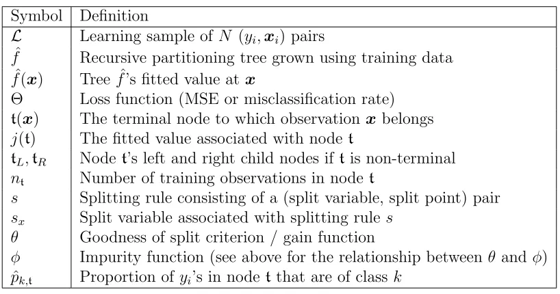
Figure 1.1: CART fit to the Boston Housing data. Terminal nodes are restricted to

contain no fewer than 5% of all observations. In-sample R2 = 0.8.

| rm< 6.941

lstat>=14.4

crim>=6.992

lstat>=19.85 dis< 1.986

crim>=0.6148

rm< 6.543

lstat>=9.66

dis>=4.442

age>=69.15

nox< 0.601

dis>=4.196

lstat>=7.57

lstat>=6.03 rm< 7.437

10.5614.44 14.9

15.9619.8319.51

19.56 21.5

21.9521.1723.65 27.02

25.9830.13 32.11 45.1

Now because ˆf is a binary tree we can find ˆf(x) simply by applying a series

of rules. We write Bt to denote the sequence of split variables leading to node

t. Let t be the left-most terminal node. Then the sequence of splits leading to t

is therefore (rm,6.941), (lstat,14.4), (crim,6.992), (lstat,19.85) corresponding to

Bt ={rm,lstat,crim,lstat}. As noted previously, the fitted value of an observation

for which x∈t is explained by simply enumerating this sequence of rules:

“If the rm is less than 6.94, lstat is greater than 14.4, crim is greater

than 6.99, andlstatis greater than 19.85, then the fitted value is 10.56.”

The node is at depth four and so the explanation is an intersection of four rules. Now

clearly the more features used to reach a given terminal node t, the more difficult it

is to summarize the partition of X t describes. Note, however, that in this case the

explanation can be simplified by condensing the two statements aboutlstatinto the

single rule “lstatgreater than 19.85.” Similarly, the right-most terminal node can be

described with the single rule “if rmexceeds 7.437, then ˆf(x) is 45.1,” despite the fact

(22)

More generally, because terminal nodes represent contiguous regions of X, depth

d terminal nodes whose branches split on fewer than dseparate predictors can be

in-terpreted as the intersection of fewer thandrules. Put differently, sequential splits on

the same variable are easily explained because they predictyusing a single dimension

of X. In the most extreme case, therefore, a node whose branch uses only a single

variable corresponds to a contiguous region inX defined by a single dimension. This

yields a single-rule explanation of the fitted value, regardless of the depth at which the

node appears. Additionally, if these sequential splits uncover a monotonic

relation-ship between the split points and fitted values, the explanation becomes easier still.

In this sense, Breiman’s concept of “simple characterizations” ofX can be understood

in part by the extent to which a tree’s branches tend to reuse split variables.

1.3 Penalized Split Criteria for Interpretable Trees

1.3.1 Penalized Split Criteria

As we have seen, branches comprising small subsets of predictors are more

inter-pretable than those containing new predictors at each split point. With this in mind,

the criterion presented in this section encourages interpretable trees by penalizing

splits that extend the set of features used in a given branch. Under this criterion the

chosen splits? is not necessarily the one that most reduces impurity, which obviously

worsens the extent to which the tree fits the data. Nevertheless, it is encouraging

that the presence of a single split which minimizes impurity does not imply the

ab-sence of other suitable split options, even if minimizing impurity is the sole objective.

Readers familiar with the literature will recall that the chosen split s? _{can be quite}

unstable, and that in reality many different splits may result in similar values of the

(23)

follows.

At any given node, there may be a number of splits on different variables, all of which give almost the same decrease in impurity. Since the data are noisy, the choice between competing splits is almost random.

As pointed out by many authors, the variability of CART splits is a drawback from

a bias-variance perspective (see Breiman (1996a) and Hastie et al. (2009)). Here

we focus on interpretability, and in the following sections we show how the presence

of multiple splits with similar φ values can actually be advantageous for growing

interpretable trees.

The central idea is that if choosing a particular split rule from a set of competing

rules with similarφ’s is “almost random” as Breiman et al. (1984) asserts, then

select-ing the most interpretable one from the set rather than that which strictly maximizes

the gain function should yield a tree that both fits the data and is easy to explain.

To that end, given a non-negative penalty function γ for splitting t as per rule s, we split according to

s? = arg max s∈S

{θ(t, s)−γk(t, s,Bt)}, (1.6)

where the k refers to a penalization constant to be discussed shortly. As before, Bt

is the ordered list of split variables used in the branch of the tree leading to t. The

algorithm is still recursive but is now path dependent. Particular definitions of γ are

the subject of Sections 1.3.2 and 1.3.3. Note that while penalizing the split criterion

as in 1.6 is related to variable costs insofar as both methodologies can reduce the

subset of variables a tree uses, variable costs must be specified by the user a priori.

In contrast, the methodologies described herein are completely automatic.

The constant k is a tuning parameter that controls the tradeoff between the gain

function and the penalty: high k values will correspond to a strong preference for

(24)

splits with less than the maximal gain can result in reduced fit in terms of R2 _or

the misclassification rate. Nevertheless, as we shall see in the subsequent sections, in

many cases the reduction is not drastic and could well be worth the improvement in

interpretability. Of course the nature of the tradeoff varies with the dataset, and so

it is advisable to run the algorithm for a variety ofk values. If we do not wish to use

the tree for out-of-sample prediction this could very well be the end of the story – we

simply choose the tree that yields the best combination of fit and interpretability for

the problem at hand.

If a more systematic approach is desired, a natural procedure is to select the

highest k that results in a global fit no worse than that of the unpenalized tree’s

by some predefined fraction. We define this formally as follows. Recalling that L

denotes our learning sample of N (yi,xi) pairs, we write Θ[ ˆf ,L] to denote tree ˆf’s

loss evaluated on L. At this point we only consider in-sample metrics (Section 1.4

discusses penalization’s out-of-sample performance), and so L serves as ˆf’s training

data as well. In regression, for example, we take

Θ[ ˆf ,L] =X i∈L

(yi−fˆ(xi))2, (1.7)

the usual squared-error loss. For convenience, in plots and tables we re-express this

quantity as R2 _{in order to remove the scale of} _{y. In classification we let Θ be the}

misclassification rate (MR). Writing ˆfk indicate a tree grown with a particular tuning

parameter, we choose the parameter k? as per

k? = max k

n

k: Θ[ ˆfk,L] ≤ (1 +c) Θ[ ˆf0,L] o

, (1.8)

where c >0. That is, we choose the largest k that still results in a tree whose loss is

(25)

k’s for the penalized trees displayed in Sections 1.3.2 and 1.3.3 are chosen according

to this procedure with c= 0.10.

Note that in regression θ(t, s) is the decrease in mean squared error, which is

dependent on the scale of the response variable. Penalizing MSE directly means the

choice of k in (1.6) is dependent on the level of y in a given problem. To make k

values comparable across datasets, in the sections below we re-express θ to measure

the proportional improvement in impurity gained by splitting t as per rule s. The details of the scaling vary with the impurity function and are deferred to Appendix

A.1.1, but in each case we ensure that θ≤1 for all s∈ S, we prefer splits with larger

θ, and we are indifferent between splitting and not splitting when θ = 0. Herein we

assume scaled gain functions, letting us restrict k to the interval [0,1].

1.3.2 New Variable Penalty

The first of our new methods is targeted at limiting the number of predictors used

to reach a tree’s terminal nodes. As we have described, the more variables used to

reach t the more complex the explanation of t’s subset of X, and so in cases where

many splits offer nearly the sameφit may be preferable to choose a split on a variable

already used inBt.

Letting sx ∈ {1, ..., p} denote rule s’s split variable, the new variable penalty is written

γk(t, s,Bt) = k1(sx ∈/ Bt). (1.9)

Hence if s introduces a new variable into the branch the penalty is k. If s uses a

previously used variable, there is no penalty. Thus splits that introduce new variables

must improveθby at leastkin order to be selected, whereas splits on old variables can

be selected so long as the improvement is greater than 0. Whatever the split criterion,

(26)

not introduce new variables into the branch. This penalty (and more generally any

penalized criterion written in the form of Equation 1.6) can be made compatible with

any suitably scaled split criterion. In the following we demonstrate the performance

of the penalty (1.9) on the previously used datasets for a selection of split criteria.

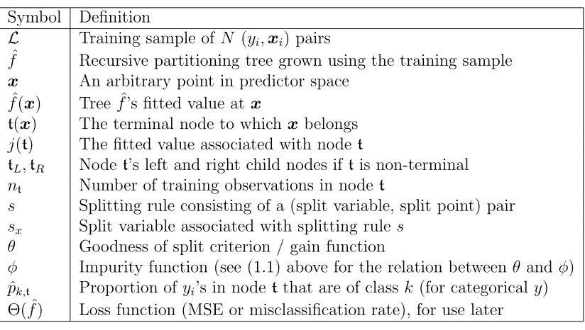
In Figure 1.2 we compare trees grown to the Boston Housing data using (1.3), the

conventional CART regression criterion, with and without the new variable penalty.

First we note that despite the penalization, the R2 values are comparable. The trees

are equivalent up to the third level of splits, where the conventionally grown tree

(Figure 1.2a) introduces crim into the leftmost branch. All told, the unpenalized

tree uses as many as five variables in reaching a terminal node, whereas the penalized

tree (Figure 1.2b) never uses more than three. This makes a considerable difference

when one attempts to explain the fit at a particular node. For instance, the region

described by the bottom-left node of the penalized tree (for which j(t) = 20.63)

might be described by saying “if rm is between 5.85 and 6.54 and lstat is between

9.66 and 14.4, the fitted value is 20.63.” Constructing an analogous description of the

bottom-left node of the unpenalized tree is substantially more tedious.

Figure 1.2: CART applied to the Boston Housing data.

(a) Unpenalized

In-sampleR2 = 0.8

| rm< 6.941

lstat>=14.4

crim>=6.992

lstat>=19.85 dis< 1.986

crim>=0.6148

rm< 6.543

lstat>=9.66

dis>=4.442 age>=69.15

nox< 0.601

dis>=4.196

lstat>=7.57

lstat>=6.03 rm< 7.437

10.5614.44 14.9

15.9619.8319.51

19.56 21.5

21.9521.1723.65 27.02

25.9830.13 32.11 45.1

(b) New Variable Penalty (k? = 0.27)

In-sampleR2 = 0.79

| rm< 6.941

lstat>=14.4

lstat>=19.83

nox>=0.6695 rm>=6.178

lstat>=16.09

rm< 6.543

lstat>=9.66

rm< 5.848

lstat>=11.69

lstat>=7.195

lstat< 8.545

lstat>=6.03 rm< 7.437

10.34 15.27 15.41

17.15 18.66 19.76

20.63 21.39 21.66 24.77 24.75

(27)

As per (1.8), 0.27 is the maximal value for k that achieves a mean-squared error

no more than 1.10 times that of the traditionally grown tree. Of course depending

on how the analyst values fit versus interpretability, he can use higher values for k

resulting in even fewer variables used and a commensurate increase in in-sample MSE

(decrease in R2_{). For instance, Figure 1.3 uses} _k ₌ _{.4, and largely describes the}

monotonic relationship between average home size and median prices.

Figure 1.3: CART fit to the Boston Housing data with the New Variable Penalty

(k?_{=0.4). In-sample} _R2_=0.67.

| rm< 6.941

rm< 6.546

rm< 5.858

rm< 5.548

rm< 5.758

rm< 6.049

rm>=5.909

rm< 5.979

lstat>=14.44

lstat>=17.91 lstat>=9.98

rm>=6.258 rm< 6.676

rm< 7.437

14.89

17.23 17.8

18.44 18.75 20.8

13.89 16.59 21.02

23.65 24.79 24.89 25.95

32.11 45.1

The penalization framework applies to split criteria besides the usual CART

methodology. As an example, we consider the one-sided high means criterion

de-scribed in Buja and Lee (2001). Unpenalized, this method chooses the split s that

isolates the single child node with the highest mean:

s?_hm= arg max s∈S

{max

s {y¯tL,y¯tR}}. (1.10)

An overview of the one-sided procedures introduced in Buja and Lee (2001) is

con-tained in Appendix A.1.2. Applying this procedure to the Boston Housing data yields

the left tree in Figure 1.4, with the penalized version appearing on the right. TheR2

values are comparable, but the penalized tree is considerably simpler as it involves

only three predictors instead of six. The trees use only rm and lstat until the

(28)

on nox and tax, whereas the penalized tree uses only crim and lstat, leaving the

monotonic relationships undisturbed.

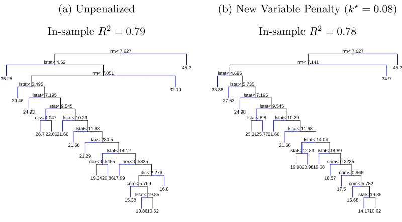
Figure 1.4: One-sided High-Means fit to the Boston Housing data.

(a) Unpenalized

In-sampleR2 _{= 0}_.₇₉

| rm< 7.627 lstat< 4.52 rm< 7.051 lstat< 5.495 lstat< 7.195 lstat< 9.545 dis< 4.047 lstat< 10.29

lstat< 11.68 tax< 280.5

lstat< 14.12 nox< 0.5455 nox< 0.5835

dis< 2.279 crim< 5.769 lstat< 19.85 36.25 29.46 24.93 26.7 22.0621.66 21.66 21.29 19.3420.8617.99 15.38 13.8610.62 16.8 32.19 45.2

In-sampleR2 _{= 0}_.₇₈

| rm< 7.627 rm< 7.141 lstat< 4.695 lstat< 5.735 lstat< 7.195 lstat< 9.545 lstat< 8.8 lstat< 10.29

lstat< 11.68 lstat< 14.04 lstat< 12.83 lstat< 14.89

crim< 0.2235 crim< 0.966 crim< 5.782 lstat< 19.85 33.36 27.53 24.98 23.3125.7721.66 21.66 19.9820.9819.68 18.57 17.5 15.68 14.1710.62 34.9 45.2

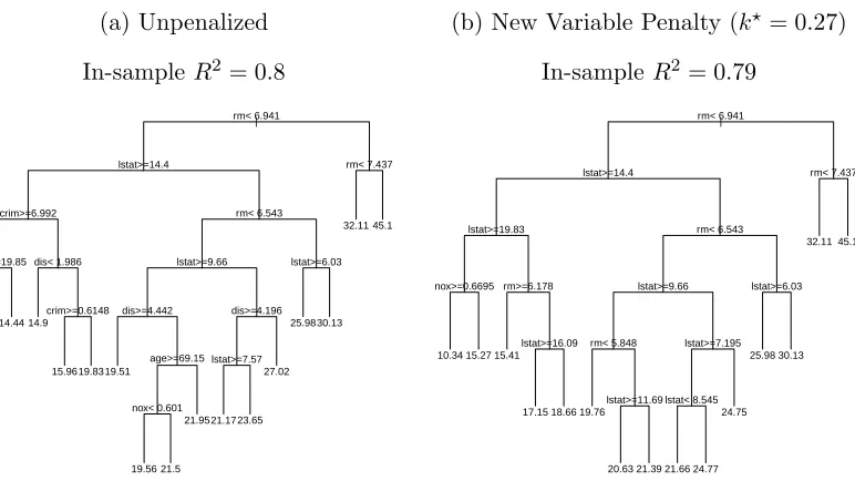
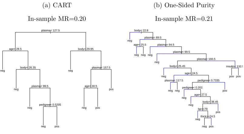
Turning to classification, Figure 1.5 combines the new variable penalty with Buja

and Lee (2001)’s one-sided purity criterion, which splits so as to isolate the single

child node with minimum Gini (minimum classification impurity). Comparing the

penalized tree in Figure 1.5b with its unpenalized counterpart in Figure 1.5a, we see

that we can achieve less than 10% increase in the in-sample misclassification rate

while reducing the total number of predictors used from seven to two. Here applying

the new variable penalty allows us to uncover high-purity regions of X that are also

relatively simple to interpret.

1.3.3 EMA-Style Penalty

Let us consider more closely the four leaf nodes at depth 6 in the penalized tree

in Figure 1.2b (the leftmost of these leaf nodes has j(t) = 20.63). Using the new

(29)

Figure 1.5: One-Sided Purity fit to the Pima Indians Diabetes data with and without

the New Variable Penalty. (MR = Misclassification Rate)

(a) Unpenalized

In-sample M = 0.21

| body< 22.8

plasma< 89.5 age< 25.5 plasma< 94.5

plasma< 99.5

plasma< 166.5 body< 25.45

age< 24.5

plasma< 117.5 pedigree< 0.7335 pedigree< 0.202 age< 27.5 body< 38.45 bp>=79 thick>=24.5 insulin< 132.5 neg 57/2 neg 45/0 neg 38/7 neg 35/4 neg 35/5 neg 42/4 neg 37/4 neg 37/15 neg 37/14 neg 30/12 neg 22/16 neg 25/20 pos 21/29 pos 13/26 pos 15/42 pos 8/33 pos 3/35

In-sample MR = 0.23

|

body< 22.8 body< 25.45

body>=24.35 body< 26.75 body< 27.85 body< 29.85 plasma< 87.5 plasma< 165.5 plasma< 99.5 plasma< 107.5 body< 42.2 plasma< 147.5 body>=37.25 plasma< 129.5 body>=34.05 neg

neg neg neg neg neg neg neg neg neg neg neg pos pos pos pos

This represents an improvement over the corresponding branches in the unpenalized

tree in Figure 1.2a that eventually split on dis, ageand nox. Nevertheless, the fact

that the predictors are interleaved makes constructing a more precise explanation

difficult. Longer sequences of splits on the same variable would enable us to interpret

the fits as monotonic relationships inrm and/or lstat, but here that is not possible.

This should be no surprise – while (1.9) expresses our preference for using fewer

variables, it is indifferent to the ordering of variables in a given branch.

Our second method targets both preferences. Here we penalize not only new

variables, but also favor variables used recently in the branch. We achieve this by

employing an exponential moving average-style (EMA) penalty, defined as:

γk(t, s,Bt) =

d−1 X

j=0

1(sx 6=sj)k(1−k)(d−1)−j ford >0, (1.11)

and otherwise 0. As before,k ∈[0,1] is the user-specified penalty constant and sx is

(30)

depth ofBt’s nodes, and sosj is the split variable inBt at depthj. The branches we

last discussed from Figure 1.2 have s0=rm, s1=lstat and s2=rm, for instance. Here

d is the depth of the branch not including the proposed split, or equivalently, the

number of nodes in Bt. Hence when considering candidates for the second split in a

branch we have d= 1. Obviously when considering the root split there should be no

penalty (nor does (1.11) make sense), and so we setγ = 0.

Setting aside the notational details, we see that (1.11) is an exponential moving

average of indicator functions. The j-th indicator is 1 if s’s split variable is different

from the variable used at depth j. If s splits on the same variable, as we prefer,

the indicator is 0. Further, as j → 0 we know k(1−k)(d−1)−j _{decreases, and so}

the weights attenuate as we move up Bt towards the root. This conforms to our

preferences: splitting a node on a different predictor from its parent is a graver offense

than splitting on a different predictor from the root. Correspondingly, the former

infraction contributes more to γ than the latter. Lastly we note that setting k = 0

recovers the unpenalized version of the splitting criterion.

Figure 1.6 displays a regression tree grown using the CART procedure but with

the EMA-style penalty. The unpenalized version of this tree appears in Figure 1.2a.

Immediately we see that the new penalty eliminates the previously observed tendency

for consecutive nodes to switch between splitting on rm and lstat. The benefit is

that the fit is easily explained primarily in terms of two monotonic relationships: for

areas with very large homes (rm>6.94) prices are monotonically increasing in home

size, and for the remaining areas prices are decreasing in lstat. A very similar story

emerges from using the EMA penalty with the high-means criterion, as displayed in

Figure 1.7. In fact, some of the nodes in these trees characterize the exact same

(31)

Figure 1.6: CART fit to the Boston Housing data with the EMA-Style penalty (k? =

.15). In-sampleR2 = 0.77. In comparison with the unpenalized version in Figure 1.2,

this tree uses only two predictors.

| rm< 6.941 lstat>=14.4

lstat>=19.83 lstat>=5.41 lstat>=9.95

rm< 7.437

12.35 16.95

20.69 24.17 29.94

32.11 45.1

Figure 1.7: High-Means fit to the Boston Housing data with the EMA penalty

(k?_{=.01). In-sample} _R2 _{= 0.78.}

|

rm< 7.627

lstat< 4.52

rm< 7.051

lstat< 5.495

lstat< 7.195

lstat< 9.545

lstat< 8.8 lstat< 10.29

lstat< 11.68

lstat< 14.04

lstat< 12.83 lstat< 14.89

crim< 0.2235

crim< 0.966

lstat< 18.93

lstat< 22.67 36.25

29.46

24.93

22.66 25.77 21.66

21.66

19.98 20.98 19.68

18.57

17.5

15.11

13.26 11.07 32.19

45.2

In Figure 1.8 we apply the the EMA penalty to the Pima Indians data and Buja

and Lee (2001)’s one-sided extremes criteria. This procedure chooses the split that

results in the single child node with the highest sample proportion of a specified

class. Here we search for regions of X associated with high incidence of of diabetes.

From previous examples we know that this dataset can withstand very high penalties

before the misclassification rate breaks down. Hence in this example we setcto 0 and

(32)

tree, in comparison, never uses the same variable more than twice consecutively and

employs seven predictors in all. Figure 1.9 displays the one-sided purity tree with

and without the EMA penalty when c= 0.10.

Figure 1.8: One-Sided Extremes fit to the Pima Indians data with and without the

EMA penalty. Figure 1.8b uses the EMA penalty with the highest penalty parameter

such that the penalized tree’s misclassification is no higher than that of the

unpenal-ized tree. Note the penalunpenal-ized tree uses only plasma, whereas the unpenalized tree

uses 7 predictors.

(a) Unpenalized

In-sample MR = 0.25

| plasma< 166.5 plasma< 154.5 body< 42.85 plasma< 143.5 pedigree< 0.9325 pregnant< 9.5 pregnant< 6.5 plasma< 130.5 age< 39.5 age< 30.5 pedigree< 0.633 plasma< 118.5 thick< 31.5 plasma< 107.5 body< 30.05 insulin< 132.5 neg 86/0 neg 38/1 neg 37/3 neg 35/5 neg 34/7 neg 30/8 neg 34/11 neg 28/16 neg 29/16 neg 39/22 neg 21/17 neg 21/17 neg 25/23 pos 19/24 pos 13/30 pos 8/33 pos 3/35

(b) EMA Penalty (k? _{= 0}_.₇₀₎

In-sample MR = 0.25

(33)

Figure 1.9: One-Sided Purity fit to the Pima Indians data.

(a) Unpenalized

In-sample MR = 0.21

| body< 22.8

plasma< 99.5

age< 24.5

plasma< 117.5 pedigree< 0.7335 pedigree< 0.202 age< 27.5 body< 38.45 bp>=79 thick>=24.5 insulin< 132.5 neg 57/2 neg 45/0 neg 38/7 neg 35/4 neg 35/5 neg 42/4 neg 37/4 neg 37/15 neg 37/14 neg 30/12 neg 22/16 neg 25/20 pos 21/29 pos 13/26 pos 15/42 pos 8/33 pos 3/35

(b) EMA Penalty (k? = 0.03)

In-sample MR = 0.23

| body< 22.8

plasma< 99.5

age< 24.5 plasma< 117.5 plasma< 153.5

plasma< 106.5 pedigree< 0.7335 insulin< 132.5 neg 57/2 neg 45/0 neg 38/7 neg 35/4 neg 35/5 neg 42/4 neg 37/4 neg 37/15 neg 32/15 neg 108/86 pos 10/30 pos 13/28 pos 8/33 pos 3/35

1.4 Out of Sample Performance

We have seen that one-sided split criteria and penalization often yield more

inter-pretable trees than the traditional CART methodology with only modest sacrifices

in in-sample loss, Θ. Until now we have computed loss over our learning sample L,

but naturally it is important to understand how these techniques fare on new data,

znew _{= (y}new_,_xnew_{), as well. To that end, in this section we study the impact of the}

various techniques for growing ˆf on the risk, defined by

R=

Z

znew

Z

L

Θ[ ˆfL,(ynew,xnew)] dP(L)dP(znew). (1.12)

We write ˆfL to emphasize that the fitted tree is a function of the training sample

L. In general our results suggest that applying an interpretability penalty to a given

splitting criterion has very little impact on out-of-sample loss in comparison with the

(34)

a variety of splitting methods. In the remainder of this section we discuss these results

in greater detail.

As we have neither true distribution functions nor an elegant form for the fitting

procedure L →fˆL at our disposal, we study (1.12) using the “out-of-bag”

generaliza-tion error estimate discussed in Breiman (1997). For each dataset we takeB bootstrap

samples L1, ..., LB from L. Let the bootstrap samples be indexed by b ∈ {1, . . . B}.

Observations in L not in Lb are set aside as holdout data, Hb. Using a tree fitting

procedure F we fit a tree to each sample. Then for each tree we evaluate loss Θ on

its holdout data Hb, yielding an estimate of generalization error ˆΘb. The procedure

is given completely by Algorithm 1 in Appendix A.1.3. We then approximateR with

the mean of the ˆΘ values:

ROOB = 1 B

B

X

b=1

ˆ

Θb. (1.13)

In Algorithm 1 F represents the fitting procedure. Here we use both CART and

the one-sided splitting criteria introduced in Buja and Lee (2001). One-sided splitting

criteria are written

θOS(t, s) = φ(t)−min{φ(tL), φ(tR)}, (1.14)

with s? ∈ S still chosen by maximizing the gain function as in (1.1). In replacing

(1.2)’s weighted sum over child nodes with minimization, (1.14) favors splits with low φ on the left at the expense of high φ on the right and vice versa, regardless of

relative node size. Appendix A.1.2 describes how the high means and one-sided purity

methodologies seen previously fit into this framework in addition to summarizing the

remainder of the procedures described by Buja and Lee (2001).

Turning to the interpretability penalties, the reader will recall that we set the

(35)

the most interpretable tree that still achieves a certain fraction of the unpenalized

method’s performance on the data at hand. When we write “penalization method” or

“penalization procedure” we mean a particular penalization function coupled with our

rule for choosing k. To study the penalties’ out-of-sample performance, we compute

the out-of-bag error estimate as before but apply (1.8) to each bootstrap learning

sample. By this we mean that theF from Algorithm 1’s lineTb ←F(Lb) includes the

search over possiblekvalues. Hence ˆΘ remains a metric of out-of-sample performance.

Starting with Table A.3 in Appendix A.1.4 we display the estimated loss obtained

from applying each splitting criterion and penalty method combination (including

no penalty) to our datasets. We set B = 100 and k = (0.01,0.02, . . . ,0.99). For the

penalized methods, the column entitled “Averagek?_{” reports the mean}_k_{value selected}

across the B bootstrap samples. Low averagek? _{values suggest that on average, the}

splits chosen by the non-penalized methods have relatively few competitors in terms

of reducing loss. The two wine datasets are examples of this – apparently in predicting

wine quality, swapping the “best” split for a more interpretable one coincides with a

substantial increase in MSE. In contrast, highk?_{, such as those found on the “ankara}

dataset”, suggest that many predictors yield similar performance.

Generally, the results suggest that our method for choosingk? _{results in penalized}

trees whose risk remains quite close to that of the unpenalized methods. For example,

Table A.3 shows that on our ten benchmark regression tasks, penalized CART’s

esti-mated risk is always less than 10% higher than CART’s. In fact over all 2×4×10 = 80

possible penalty/criterion/dataset combinations in Tables A.3-A.6, only one has an

increase in MSE above 10%. The evidence from classification is similar – in just one

case does applying a penalty increase a splitting criterion’s holdout misclassification

rate by more than 10%. In many cases misclassification rate decreases.

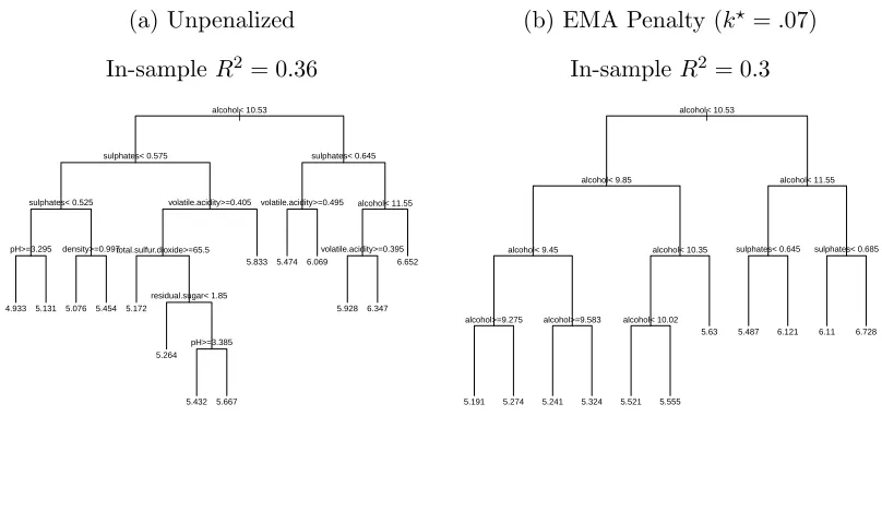
Moreover, the gains in interpretability can be substantial amounting to a “free

(36)

predict each wine’s (ostensibly) human-labelled quality score using predictors that

measure various aspects of the wine’s chemical composition. Figure 1.10 displays the

unpenalized CART tree on the left and the EMA penalized tree on the right. We

select k? ₌ _{.07 by our usual method with} _c _{= 0.10. The unpenalized tree uses as}

many six predictors in a branch, whereas the penalized tree uses only alcohol and

sulphates in the entire tree. Moreover, the right tree’s fit is easily described as an

increasing relationship between alcohol and quality for low values of alcohol and

an increasing relationship betweensulphates and quality for higheralcoholvalues.

The EMA penalty’s out-of-bag risk estimate is only 1.8% higher than that of CART’s

(see Table A.3), suggesting we can replace the CART fit with a far more interpretable

tree that we can expect to perform essentially just as well on new data.

Figure 1.10: CART fit to the Red Wine data.

(a) Unpenalized

In-sampleR2 = 0.36

|

alcohol< 10.53

sulphates< 0.575

sulphates< 0.525

pH>=3.295 density>=0.997

volatile.acidity>=0.405

total.sulfur.dioxide>=65.5

residual.sugar< 1.85

pH>=3.385

sulphates< 0.645

volatile.acidity>=0.495 alcohol< 11.55

volatile.acidity>=0.395

4.933 5.131 5.076 5.454 5.172

5.264

5.432 5.667

5.833 5.474 6.069

5.928 6.347 6.652

(b) EMA Penalty (k?=.07)

In-sampleR2 = 0.3

|

alcohol< 10.53

alcohol< 9.85

alcohol< 9.45

alcohol>=9.275 alcohol>=9.583

alcohol< 10.35

alcohol< 10.02

alcohol< 11.55

sulphates< 0.645 sulphates< 0.685

5.191 5.274 5.241 5.324 5.521 5.555

5.63 5.487 6.121 6.11 6.728

1.5 Conclusion

This chapter describes penalization methods for growing classification and regression

trees targeted at settings where interpreting the resultant tree is particularly

(37)

subset of variables used in each branch. By requiring that less interpretable candidate

splits decrease the parent node’s impurity more than others, penalization allows us

to favor interpretability when many splits offer similar improvements. Interestingly,

it is the tendency for many splits to offer very similar decreases in impurity – one of

CART’s perceived disadvantages – that makes this possible.

Using real datasets we show that the penalty functions can indeed result in trees

that are substantially easier to explain than their unpenalized counterparts. This

observation holds for a variety of splitting criteria and across both classification and

regression problems. Further, our study suggests that tuning a penalization parameter

to maintain in-sample loss no more than a fraction c of that of the unpenalized

procedure’s results in generalization error that is almost always within 100c% of the

unpenalized method’s. That is, in nearly all cases the penalization techniques return

a more interpretable fit for very little increase in out-of-sample loss, yielding a “free

lunch” of sorts. This raises a number of interesting questions, such as why this might

be the case, whatX designs it is true for, or if further gains can be made by explicitly

tuning penalty parameters to minimize holdout loss.

Acknowledgements

We thank Ed George and Abba Krieger for their insightful comments on this project.

We also thank Richard Berk for his thorough reading and substantive edits on an

(38)

2

Software for Interpretable Classification and

Regression Trees

Abstract

This chapter describesitree, anRpackage for fitting for classification and regression

trees. Besides the familiar CART methodologies, the package implements splitting

criteria and risk estimation techniques that aim to enhance a tree’s visual

inter-pretability. For the procedures unique to itree we give a methodological overview,

present illustrative examples, and demonstrate itree’s usage.

2.1 Introduction

Recursive partitioning trees are a popular supervised learning technique. Indeed, the

rich variety of Rpackages implementing ideas that descend from Breiman et al. (1984)

or Quinlan (1986) attests to the community’s continued interest in these methods. In

this chapter we describe itree, an addition to R’s tree-fitting landscape that

imple-ments a variety of methods useful for growing interpretable and/or parsimonious trees.

(39)

usual CART methodology, the software extends and modifies rpart, the excellent

package for classification and regression trees.

From a methodology perspective, the procedures unique to itree are naturally

organized into three groups. The first set of techniques was first introduced in Buja

and Lee (2001) and concern splitting criteria that induce imbalanced trees. Buja and

Lee (2001) refers to them collectively as one-sided procedures. The second group is based on the work of Goldstein and Buja (2013), which discusses ways to favor splits

that restrict the subset of predictors used in a given branch of a tree. Goldstein and

Buja (2013) achieves this by introducing penalties into the splitting criteria. As we

will see, itree implements these penalties as to work with any valid splitting rule

whether CART, one-sided, or even user-defined. The third concerns a technique first

illustrated in Breiman (1997) for using the out-of-bag observations created by bagging

to assess a tree’s local out-of-sample performance. Here we extend the ideas found in

Breiman’s paper both by generalizing the methodology to classification and allowing

the user to plot the metric alongside a tree’s fitted values. The result is a visual

diagnostic for assessing a method’s out-of-sample performance over different regions

of the feature space.

The chapter is organized as follows. In Section 2.2 we provide a brief CART

overview and introduce some notational conventions. Sections 2.3, 2.4 and 2.5

ad-dress the one-sided criteria, penalization, and local risk procedures in turn. In each

section we demonstrate the package’s use with code snippets alongside the

method-ology discussion. Section 2.6 contains concluding remarks.

2.2 Overview of Classification and Regression Trees

Where possible we follow the notation used in Breiman (1996b). For convenience

(40)

recall that given a learning sampleLofN pairs (yi,xi) from an arbitrary distribution,

the algorithms described in Breiman et al. (1984) output a recursively grown binary

tree ˆf(x). Here ˆf is called a classification or regression tree and the loss function Θ is

taken to be the misclassification rate or mean-squared-error (MSE, herein) depending

on whether y is categorical or continuous, respectively.

For anyx, ˆf(x) is given by the mean (for regression) or most common (in

classifi-cation)yi value over alli∈ L that are in the same terminal node as x, denoted t(x).

In either case, all observations in a given nodet share a single fitted value, which we

denote j(t) herein.

To each non-terminal node, a splitting rule s is applied, defined by a pair (x, t) consisting of a variable xand a split location t on that variable. The rules= (x1,0),

for instance, divides the nt observations int into two subsets, depending on whether

each x vector has a positive first coordinate. We call sx = x1 the split variable

and 0 the split point. The growing phase consists of selecting the best split for the observations in t and then sending them to the appropriate child nodes, where the

recursion begins anew.1 _{Proposing new meanings of “best split” is the subject of}

sections 2.3 and 2.4.

CART determines the “best s” by the goodness of split criterion or gain function θ(t, s) which quantifies the benefit of splitting nodet as per rule s. Each node splits

at

s? = arg max s∈S

θ(t, s), (2.1)

meaning we choose the split that maximizes the split criterion, where S is the set of

all possible splits including no split. θ is of the form

θ(t, s) =φ(t)−

ntL nt

φ(tL) + ntR

nt

φ(tR)

, (2.2)

1_{To lessen overfitting, it is common practice to set a minimum node size and/or prune the tree}

(41)

wheretLandtR are the left and right child nodes defined bys, andφis the loss or

so-calledimpurity function. By multiplyingφLandφRby the proportion of observations in the left and right child nodes,θ(t, s) measures the average improvement in impurity

from splitting tas per rule s.

As mentioned above, in regression settings we wish to minimize MSE and so we

set

φR(t) = 1 nt

X

i∈t

(yi−j(t))2 (2.3)

Recall that in regression we set j(t) to the sample mean of the in-node y values, and

so readers will quickly identify (2.3) as t’s (biased) sample variance, ˆσ2(t). This is the

impurity function rpart uses when one setsmethod="anova".

For reasons that are well documented, when growing trees for classification or class

probability estimation we do not take φ to be the weighted average misclassification

error (see Breiman et al. (1984) or Buja and Lee (2001), for instance). Rather,

we use either the Gini or Cross-entropy criterion. For the K-class problem with y∈ {1,2, ...K} the Gini criterion is written

φG(t) =

X

k∈K ˆ

pk,t(1−pˆk,t) (2.4)

where ˆpk,t is the proportion of yi’s in node t’s that are of class k. Cross-entropy is

defined by

φCE(t) =

X

k∈K ˆ

pk,tlog(ˆpk,t). (2.5)

Breiman (1996b) notes that empirically, Gini tends to yield splits resulting in purer

nodes, especially whenK >2. In their informative description of theRpackagerpart,

Therneau and Atkinson (1997) comment that from a practical perspective there is

usually little difference between the methods, especially when K = 2. The rpart

(42)

do likewise; when referring to the conventional method of growing classification trees

we assume Gini impurity as defined in (2.4).

Table 2.1: Summary of Notation

Symbol Definition

L Learning sample of N (yi,xi) pairs ˆ

f Recursive partitioning tree grown using training data ˆ

f(x) Tree ˆf’s fitted value at x

Θ Loss function (MSE or misclassification rate)

t(x) The terminal node to which observation x belongs j(t) The fitted value associated with node t

tL,tR Node t’s left and right child nodes ift is non-terminal nt Number of training observations in node t

s Splitting rule consisting of a (split variable, split point) pair sx Split variable associated with splitting rule s

θ Goodness of split criterion / gain function

φ Impurity function (see above for the relationship between θ and φ) ˆ

pk,t Proportion of yi’s in node tthat are of class k

2.3 One-Sided Gain Functions

Clearly (2.2) enforces a measure of balance between the impurity in right and left

child nodes – candidate splits with low impurity on the left at the expense of high

impurity on the right will likely be passed over for splits with more even performance.

Put differently, (2.2) represents a compromise between φL andφR. Insofar as we care

about ˆf’s performance over the entire X space, as is typically the case, balance is a

virtue.

An alternative approach to growing binary trees is described in Buja and Lee

(2001). Instead of balancing a statisticφ over the left and right nodes, these methods

(43)

splitting criteria can be written

θOS(t, s) = φ(t)−min{φ(tL), φ(tR)}, (2.6)

with s? ∈ S still chosen by maximizing the gain function as in (2.1). In replacing

(2.2)’s weighted sum over child nodes with minimization, (2.6) favors splits with low φ on the left at the expense of highφ on the right, regardless of relative node size. It

is because they ignore theφ value in one of the child nodes that Buja and Lee (2001)

refer to these methods as “one-sided.”

2.3.1 One-Sided Purity

Recursively splitting as per (2.6) amounts to a greedy search for partitions of X

associated with lowφ. Ifφis a loss metric, for instance, the procedure finds partitions

of X in which f(x) is particularly well approximated by a binary tree. More simply,

this corresponds to findingxvectors whose associatedy’s are close together. To that

end, Buja and Lee (2001) proposes setting φ to be the conventional CART impurity

functions. For regression this gives us

φosp,R(t) = 1 nt

X

i∈t

(yi−j(t))2 = ˆσ2(t), (2.7)

and combined with (2.6) this yields

θosp,R(t) = ˆσ2(t)−min

ˆ

σ2(tL),σˆ2(tR) . (2.8)

Recalling that we split at the rule that maximizes θ, it is clear thats? _{is the split}

that finds the single child node with the lowest average squared-error loss.

(44)

appropri-ately. As an example, we use itree to fit both the conventional CART tree and the

one-sided purity tree to the well-known Boston Housing data, where the goal is to

fit median home prices in a census tract using a variety of predictors regarding the

homes’ average physical characteristics and locations. The code is as follows.

> library(itree)

> bh.cart <- itree(medv~.,data=bh,minbucket=25,minsplit=25,cp=0) > bh.purity <- itree(medv~.,data=bh,method="purity",

+ minbucket=25,minsplit=25,cp=0)

Note that in the first line itree figures out from medv that this is a regression

problem and chooses method="anova"for the CART tree implicitly. More generally,

readers familiar withrpart will note that the syntax and arguments are exactly the

same, save the fact that itree accepts"purity"as a valid method. In fact, in cases

where one enters a valid rpart command, itree gives the same results. Thus many

scripts written for rpart can be modified to use itree by swapping occurrences of

“rpart” for “itree” and adjusting the arguments. The call creatingbh.cartwould run

identically in rpart and give the same tree, for example.

The methods outlined in this chapter focus on tree-growing rather than pruning,

and so our convention is to cease splitting oncent reaches 5% of n. This is controlled

using theminsplitandminbucketarguments, which function identically torpart’s.

The Boston Housing data has 506 observations, hence we setminbucket=minsplit=25

above. To be clear, the 5% convention is not the default functioning of itree, hence

leaving these arguments out of the commands above would result in trees with smaller

terminal nodes. As an aside, we remark that the cp argument (identical torpart’s)

also allows for premature stopping of the tree-growing phase. See Therneau and

Atkinson (1997) for details. Its functioning is considerably more complex than the

(45)

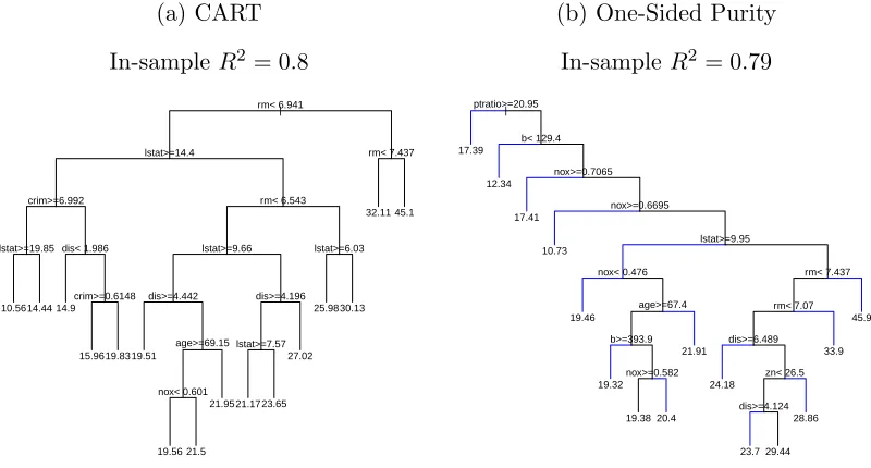
Figure 2.1 displays the result of plotting the returned objects using the usual

plot(...) command. Each subfigure’s caption shows the applicable model’s

in-sample R2_{. Note that plotting follows} _rpart_{, and so the call} _{plot(bh.cart)} _plots

bh.cart’s skeleton and text(bh.cart) then labels the nodes by printing splits and

fitted values where appropriate.

Figure 2.1: CART and One-Sided Purity applied to the Boston Housing Data.

Ter-minal nodes are restricted to contain no fewer than 5% of all observations.

(a) CART

In-sampleR2 = 0.8

| rm< 6.941

lstat>=14.4

crim>=6.992 lstat>=19.85 dis< 1.986

crim>=0.6148 rm< 6.543 lstat>=9.66 dis>=4.442 age>=69.15 nox< 0.601 dis>=4.196 lstat>=7.57 lstat>=6.03 rm< 7.437 10.5614.44 14.9 15.9619.8319.51 19.56 21.5 21.9521.1723.65 27.02 25.9830.13 32.11 45.1

(b) One-Sided Purity

In-sampleR2 = 0.79

| ptratio>=20.95 b< 129.4 nox>=0.7065 nox>=0.6695 lstat>=9.95 nox< 0.476 age>=67.4 b>=393.9 nox>=0.582 rm< 7.437 rm< 7.07 dis>=6.489 zn< 26.5 dis>=4.124 17.39 12.34 17.41 10.73 19.46 19.32 19.38 20.4 21.91 24.18 23.7 29.44 28.86 33.9 45.9

For one-sided trees, branches highlighted in blue correspond to the node generating

minimumφ. This is done using the highlight.color argument as shown below.

> plot(bh.purity,highlight.color="BLUE")

Setting highlight.color="BLACK" or highlight.color="RED" turns off

highlight-ing and highlights the branch in red, respectively.

Turning to the trees themselves, we see that despite their similar R2 _{values, these}

fits suggest very different explanations of what makes homes particularly expensive

or cheap. Immediately we see that the root splits, known to be the most stable, are

(46)

average number of rooms, rm only enters the one-sided tree in Figure 2.1b at depth

6. The one-sided tree’s root split uses pt, the parent-teacher-ratio, which does not

enter the CART tree at all. Obviously the variables used to greedily minimize CART

impurity and those used to find regions of purity are quite different.

More generally, splitting as per (2.6) yields greater variation in the depth of

termi-nal nodes, giving the one-sided tree an unbalanced look. The reason for this is clear

– should we find a bucket with high purity, it is both likely to be small and unlikely

to be split again. If our goal is to understand the subsets of X with high purity in y

this is ideal – fewer splits yield simpler, more intuitive explanations.

In classification the analogous function one-sided purity function is

φosp,C(t) =

X

k∈K ˆ

pk,t(1−pˆk,t). (2.9)

Buja and Lee (2001) only considers the two-class case in which (2.9) simplifies to

ˆ

p0pˆ1. Asitreeextends Buja and Lee (2001) to the multi-class problem, we leave the

function as written in (2.9) to make the generalization to the multi-class case obvious

– we just compute the Gini criterion at each node as before.2 Here again, substituting

(2.9) into the one-sided split criterion shows that s? _{is the split which identifies the}

child node with minimum Gini impurity.

As an example, Figure 2.2 displays a one-sided purity tree along with the usual

CART tree on the Pima Indians dataset. In this problem y ∈ {pos, neg}

depend-ing on whether the individual has diabetes and x ∈ _R8_. _{Once again, we stop}

splitting once nt is 5% of the overall n. Note that for illustrative purposes we set

method="class_purity", in which case the software does not need to make an

educated guess as to whether the user intends to fit a classification or regression

tree. In this case the diabetes variable is of class factor, and so simply passing

2_{Readers should note that this is} _one _{possible generalization to the multi-class purity problem;}

Topics in Tree-Based Methods

University of Pennsylvania

ScholarlyCommons

Topics in Tree-Based Methods

Alex Lauf Goldstein

Topics in Tree-Based Methods

TOPICS IN TREE-BASED METHODS

Alex L. Goldstein

A DISSERTATION

Statistics

For the Graduate Group in

Managerial Science and Applied Economics

Presented to the Faculties of the University of Pennsylvania

Partial Fulfillment of the Requirements for the

Degree of Doctor of Philosophy

2014

Dedication

Acknowledgments

ABSTRACT

TOPICS IN TREE-BASED METHODS

Alex L. Goldstein

Andreas Buja

Contents

List of Tables

List of Figures

1

Penalized Split Criteria for Interpretable Trees

Abstract

1.1

Introduction

1.2

Fundamentals of Classification and Regression

Trees

1.2.1

Splits and Splitting Criteria

1.2.2

CART Impurity Functions

1.2.3

Interpretability of Trees

1.3

Penalized Split Criteria for Interpretable Trees

1.3.1

Penalized Split Criteria

1.3.2

New Variable Penalty

1.3.3

EMA-Style Penalty

1.4

Out of Sample Performance

1.5

Conclusion

Acknowledgements

2

Software for Interpretable Classification and

Regression Trees

Abstract

2.1

Introduction

2.2

Overview of Classification and Regression Trees

2.3

One-Sided Gain Functions

2.3.1

One-Sided Purity