An empirical study of robust covariance estimators using biasedness

(1)

International Journal of Applied Science and Research

211

Obafemi, O.S.

Department of Mathematics and Statistics, Federal Polytechnic Ado-Ekiti, Nigeria.

IJASR 2019 VOLUME 2

ISSUE 6 NOVEMBER - DECEMBER ISSN:2581-7876 Abstract – It is generally known that in estimating location and scatter matrix of multivariate data when outliers are presents, the method of classical is not robust, because of its sensitivity to outlier; many alternative estimators that are robust have been proposed in the last decades. Some of these estimators include the Minimum Covariance Determinant (MCD), the Minimum Volume Ellipsoid (MVE), S-Estimators and Obafemi and Oyeyemi proposed estimator among others. All the methods converged on tackling the problem of robust estimation by finding a sufficiently large subset of the data. In this paper, an empirical study of the later, the classical and the two most widely used estimators is compared using biasedness. It is observed that the alternative estimator proposed by Obafemi and Oyeyemi is better because it has the least bias, virtually in all cases of non centrality parameter.

Keywords: Biasedness, Estimator, Outlier, Multivariate, covariance matrix.

INTRODUCTION

In a large survey of observations, more often than not, there is the possibility that changes in the measurement process will bring about clusters of outliers. The standard multivariate analysis methods depend on the assumption of normality which requires the use of estimates for both the location and scale parameters of the distribution. The presence of outliers in the observations may distort arbitrarily the values of the estimators and render meaningless the precision and accuracy of the results when these techniques are applied. Rocke and Woodruff (1996), opined that the problem of the joint estimation of location and shape is one of the most profound challenges encountered in robust statistics.

In statistical data analysis, quite a large number of variables are usually sampled. The first step towards obtaining a coherent analysis that will lead to estimates with good precision and accuracy is to detect outlying observations. Although outliers are usually regarded as disturbance error or noise that makes parameter estimates invalid, but it has important information which can stand as measure of quality of data or observation. Detected outliers are instrument that corrupt data which would have adversely led to model misspecification, biased parameter estimation, incorrect results, poor precision and inaccuracy. Outlier detection is one of the most important tasks in data analysis. The outliers describe the abnormality in data behaviour, such as data that deviate from the natural data variability. The cut-off value or threshold which divides data numerically is often the basis for important decision. It is therefore important to identify an outlying observation before modeling and analysis of such data (Williams et al 2002, Liu et al, 2004)

In detecting outliers in multivariate data set, the estimation of the location and scatter of the data by means of robust estimators cannot be overemphasized.

(2)

212

MULTIVARIATE OUTLIERS

In p-dimensional multivariate normal data, both the location and scatter parameters are the most concerned issue. The location is the mean vector which denotes a point in the multi-dimensional space and scatter or shape is the variance –covariance matrix of the dimensional space. In multivariate data, it is assumed that the data follows well-behaved statistical distributions. The Independent Standard Multivariate data are usually assumed to be normally distributed with zero (0) mean and units variance. Though, the assumption may not hold when the characteristics of the data complicate or confound both estimation and hypothesis testing Jackson and Chen (2004). A principal factor leading to such problems is the influence of outliers.

In literature, it has been opined that Outliers in multivariate data are more difficult to detect than outliers in univariate data, since simple graphical methods can be used to detect univariate outliers which is impossible in multivariate data. In addition, multivariate data come from many sources apart from the true population. There could be outliers due to changes of location in random directions for each outlier, there could be a cluster of outliers due to location shift in a particular direction, there could be multiple clusters of outliers in different directions, there could be outliers with the same location as good data but with more variability, or outlier can be due to shift in some of the elements of the location vector but not all of them (Rocke and Woodruff, 1996).

Rocke and woodruff, (1996) affirmed that the most difficult type of multivariate outliers detection are those good data that have the same variance – covariance matrix. Barnet and Lewies (1994) argued that the moments (Mean and variance) used in describing data are often influenced by outliers. This influence may mask true outliers and consequently hide true outliers which will incorrectly read the identification of points which are from true population as outliers.

BIASEDNESS

Volnov et al. (1996) defined the bias of an estimator as the difference between its expected value and the true value of the parameter being estimated. An estimator is called unbiased if the bias is zero, otherwise, the estimator is said to be biased. In statistics ‘bias’ is an objective property of an estimator

Bias is related to consistency in that consistent estimators are convergent and asymptotically unbiased, (hence converge to the correct value as the number of data points grows arbitrarily large), though individual estimators in a consistent sequence may be biased (so long as the bias converges to zero).

An unbiased estimator is preferable to a biased estimator, but in practice, bias estimators are frequently used generally with small bias. When a biased estimator is used bonds on the biased are calculated. A biased estimator may be used for various reasons; because an unbiased estimator does not exist without further assumptions about a population or is difficult to compute, because an estimator is median unbiased but not mean unbiased; because a biased estimator gives a lower value of some loss function or because in some cases being unbiased is too strong a condition, and the only unbiased estimators are not useful.

Medodology

Given a collection of n column vector xi in Rp , with n >p where, n is the sample and p is the dimension, in

multivariate data analysis the most basic problem is that of estimating a location vector and scatter matrix, we compare the most commonly used methods ( Classical, MCD, MVE and the Proposed alternative estimator) by measuring the biased by a given percentages of outlier.

Data sets are generated for a given contaminated fraction



as follows. The uncontaminated part Xn consists of

 

n





observations obtained from a normal distribution with parameters µ and ∑. The other part Xc contain

(3)

213

The shape matrix of ∑ is defined by







p



1

. this follows that





1

always and we can decompose the

original matrix to be







p



1

. The square root of this scalar factor, 2p 1



, is known as the scale

component of . The scatter matrix of the estimated scatter matrix S is computed as

,

1

S

G



p

and its

scale component is p

S

2 1

. The scatter matrix upon which the bias is focused is defined as

)

(

)

(

log

)

(

2 1 2 1 2 1 2 1 1    





G

S

bias

p



, p



1

log



where



1 ...



p are the eigen values of the scatter matrix.

SIMULATION PROCEDURES TO COMPARE BIAS OF THE ESTIMATES

Contaminated multivariate sample of size n from Np (µ,Ip) were simulated for p=2 and 3. The percentages of contamination used were; 3%, 10%, 20%, 33%, 40% and 50%. The magnitude of outliers, NCP considered were ; 1,2,3,4,5,6,7,8,9,10. The simulation was iterated 1000 times to attain stability. The biases of the four methods were obtained and are shown in Table i to xii with the least for each case in bold figures.

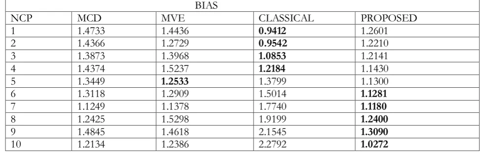
Table i. The Bias of the estimates of the four methods, when P=2, n=30, outlier 3% (1) for various levels of non centrality parameter (NCP)

BIAS

NCP MCD MVE CLASSICAL PROPOSED

1 1.4733 1.4436 0.9412 1.2601

2 1.4366 1.2729 0.9542 1.2210

3 1.3873 1.3968 1.0853 1.2141

4 1.4374 1.5237 1.2184 1.1430

5 1.3449 1.2533 1.3799 1.1300

6 1.3118 1.2909 1.5014 1.1281

7 1.1249 1.1378 1.7740 1.1180

8 1.2425 1.5298 1.9199 1.2400

9 1.4845 1.4618 2.1545 1.3090

10 1.2134 1.2386 2.2792 1.0272

Table ii. The Bias of the estimates of the four methods, when P=2, n=30, outlier 10% (3) for various levels of non centrality parameter (NCP)

BIAS

1 1.2048 1.2818 1.0221 1.2790

2 1.1968 1.1542 1.2316 1.1212

3 1.0356 1.0404 1.3876 0.9660

4 1.1791 1.1606 1.6567 1.0990

5 1.1701 1.0327 1.9612 1.0901

(4)

214

7 1.0040 1.0039 2.4678 0.8782

8 1.1039 1.1304 2.6218 1.0322

9 1.2868 1.3661 2.9301 1.0141

10 1.1415 1.1853 3.2169 0.1252

Table iii. The Bias of the estimates of the four methods, when P=2, n=30, outlier 20% (6) for various levels of non centrality parameter (NCP)

BIAS

1 1.1788 1.3211 1.0627 1.4270

2 1.3755 1.3375 1.3979 1.2582

3 1.2780 1.2805 1.7457 1.0701

4 1.0379 1.1495 1.9667 1.0582

5 1.0308 1.0254 2.5060 1.1170

6 1.2120 1.2682 2.6836 0.9041

7 1.1327 1.1599 2.9173 0.8891

8 1.2625 1.2209 3.1317 1.0582

9 1.2644 1.2578 3.3271 1.0610

10 1.1872 1.2958 3.5278 1.0291

Table iv. The Bias of the estimates of the four methods, when P=2, n=30, outlier 33% (10) for various levels of non centrality parameter (NCP)

BIAS

1 1.5527 1.6811 1.1652 1.3092

2 2.0278 1.9381 1.5350 1.6212

3 1.6586 1.6478 1.9820 0.9881

4 1.1255 1.0920 2.2868 1.1271

5 1.0632 1.0191 2.6146 0.8252

6 1.1936 1.1936 2.9627 1.4061

7 1.0438 1.0764 3.369 0.1571

8 0.9838 0.9838 3.0987 1.7740

9 1.0235 1.0235 3.8502 1.9082

10 1.0498 1.0404 3.9040 1.5921

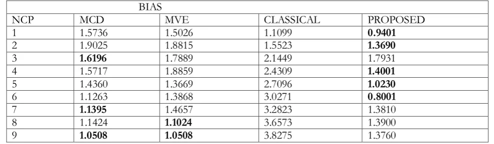
Table v. The Bias of the estimates of the four methods, when P=2, n=30, outlier 40% (12) for various levels of non centrality parameter (NCP)

BIAS

1 1.5736 1.5026 1.1099 0.9401

2 1.9025 1.8815 1.5523 1.3690

3 1.6196 1.7889 2.1449 1.7931

4 1.5717 1.8859 2.4309 1.4001

5 1.4360 1.3669 2.7096 1.0230

6 1.1263 1.3868 3.0271 0.8001

7 1.1395 1.4657 3.2823 1.3810

8 1.1424 1.1024 3.6573 1.3900

(5)

215

10 1.0242 1.0242 4.1633 1.5700

Table vi. The Bias of the estimates from the four methods, when P=2, n=30, outlier 50% (15) for various levels of non centrality parameter (NCP)

BIAS

1 1.2603 1.3796 1.0438 0.6110

2 1.5821 1.7143 1.3221 0.6651

3 2.2281 2.3634 1.8829 1.0412

4 2.6757 2.8130 2.3462 1.6050

5 3.1822 3.4496 2.7979 1.2621

6 3.8101 3.9616 3.1633 1.0842

7 4.0585 4.0697 3.3326 1.0892

8 4.0074 4.2518 3.6025 1.2751

9 4.2242 4.3843 3.7569 1.3223

10 4.5975 4.6148 4.0931 1.5001

Table vii. The bias of the estimates from the four methods, when P=3, n=30, outlier 3%(1) for various levels of non centrality parameter (NCP)

BIAS

1 1.5845 1.7497 1.1984 0.7952

2 1.8283 1.8967 1.3432 0.7571

3 1.5120 1.3498 1.4637 0.0947

4 1.8673 1.8417 1.5210 0.8662

5 1.7599 1.8167 1.8900 1.4981

6 1.5522 1.5442 2.0368 1.2321

7 1.5899 1.5737 2.1600 1.2062

8 1.8673 1.8416 2.3803 1.2751

9 1.8673 1.8416 2.5694 1.5150

10 1.6264 1.6631 2.8502 1.3221

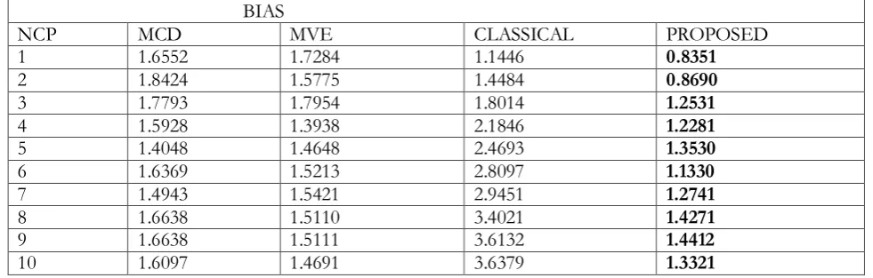
Table viii The bias of the estimates from the four methods, when P=3, n=30, outlier 10%(3) for various levels of non centrality parameter (NCP)

BIAS

1 1.6552 1.7284 1.1446 0.8351

2 1.8424 1.5775 1.4484 0.8690

3 1.7793 1.7954 1.8014 1.2531

4 1.5928 1.3938 2.1846 1.2281

5 1.4048 1.4648 2.4693 1.3530

6 1.6369 1.5213 2.8097 1.1330

7 1.4943 1.5421 2.9451 1.2741

8 1.6638 1.5110 3.4021 1.4271

9 1.6638 1.5111 3.6132 1.4412

(6)

216

Table ix The bias of the estimates of the four methods, when P=3, n=30, outlier 20 %( 6) for various levels of non centrality parameter (NCP)

BIAS

1 2.0101 1.9204 1.3088 1.0861

2 2.0775 1.9318 1.9273 1.0532

3 1.4767 1.5852 2.2294 1.3571

4 1.3036 1.3653 2.5665 1.3912

5 1.7623 1.5861 2.9743 1.4440

6 1.3634 1.3950 3.3426 1.2990

7 1.4623 1.4732 3.6600 1.2070

8 1.5982 1.3968 3.9538 1.4211

9 1.6003 1.3966 4.1726 1.4211

10 1.4718 1.4978 4.3159 1.5530

Table x. The bias of the estimates of the four methods, when P=3, n=30, outlier 33 % (10) for various levels of non centrality parameter (NCP)

BIAS

1 1.9643 1.8653 1.3710 0.7861

2 2.2351 2.2146 1.9206 1.0781

3 1.9893 2.6291 2.3010 1.5032

4 1.4080 1.8071 2.9245 1.7361

5 1.5853 1.8356 3.1550 1.7120

6 1.3135 1.6770 3.5443 1.6851

7 1.3598 1.3598 3.8317 1.7081

8 1.5932 1.5209 4.2213 2.3620

9 1.5932 1.5209 4.4495 2.4311

10 1.3813 1.3815 4.6102 2.0981

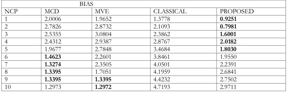
Table xi The bias of the estimates of the four methods, when P=3, n=30, outlier 40%(12) for various levels of non centrality parameter (NCP)

BIAS

1 2.0006 1.9652 1.3778 0.9251

2 2.7826 2.8732 2.1093 0.7981

3 2.5355 3.0804 2.3862 1.6001

4 2.4312 2.9387 2.8767 2.0182

5 1.9677 2.7848 3.4684 1.8030

6 1.4623 2.2601 3.8461 1.9550

7 1.3274 2.3505 4.0501 2.2391

8 1.3395 1.7051 4.1959 2.6841

9 1.3395 1.3395 4.4232 2.7502

(7)

217

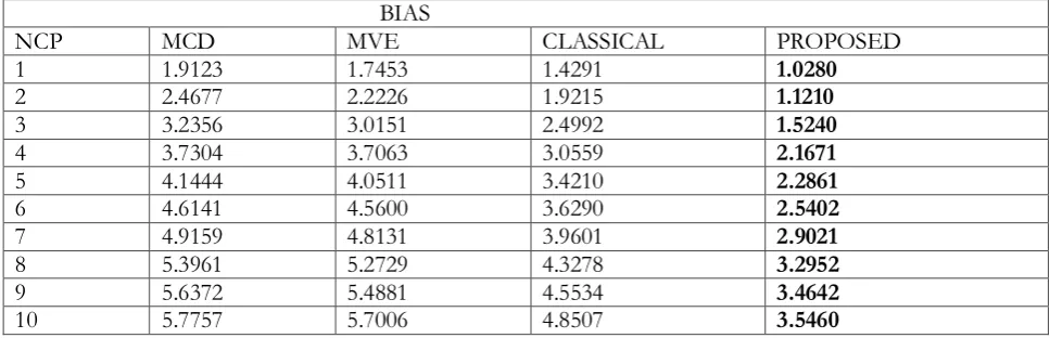
Table xii The bias of the estimates of the four methods, when P=3, n=30, outlier 50%(3) for various levels of non centrality parameter (NCP)

BIAS

1 1.9123 1.7453 1.4291 1.0280

2 2.4677 2.2226 1.9215 1.1210

3 3.2356 3.0151 2.4992 1.5240

4 3.7304 3.7063 3.0559 2.1671

5 4.1444 4.0511 3.4210 2.2861

6 4.6141 4.5600 3.6290 2.5402

7 4.9159 4.8131 3.9601 2.9021

8 5.3961 5.2729 4.3278 3.2952

9 5.6372 5.4881 4.5534 3.4642

10 5.7757 5.7006 4.8507 3.5460

The values in bold in the tables above indicated the methods with the least bias in each row.

From the results, the bias obtained using proposed methods by Obafemi and Oyeyemi alternative method is the least at all cases of percentages of outliers and NCP except in some very few cases where either the bias of other robust methods is the least, especially where the outlier percentage is very high and the NCP also very large. The bias obtained using the classical estimate is less than the bias of the estimate of the MVE and MCD whenever the NCP is 1 and 2 at all percentage of outliers. Generally the estimate of the proposed estimator is the least at almost all levels of NCP and percentages.

REFERENCES

1. Bernet and Lewis, (1994). Outliers in statistical Data. 3rd_{Edn. Wiley, New York, USA.}

2. Jackson D.A. and Chen, Y. (2004). Robust Principal Component Analysis and outlier detection with ecological data. Eviornemetics, 15(2), 159-169.

3. Liu H., Shan S., and Jiang W. (2004). On-line outlier detection and data cleaning, computer and chemical engineering, 28, 1635-1647.

4. Obafemi, O.S. and Oyeyemi, G.M. (2018): “Alternative estimator for multivariate location and scatter matrix in the presence of outlier”Annals. Computer Science Series. 16th_{Tome 2}nd_{fasc. 130-136}

5. Rocke, D. M. and woodruff, D. C. (1996). Identification of outliers in multivariate Data. Journal of American Association, 91, 1047 – 1061.

6. Rousseeuw, P. J. (1984). least modern of squares regression. Journal of the American Statistical Association, 79: 871-880

7. Voinov, V, G., Nikiliu, and Mikhail, S. (1996) Unbiased Estimators and Their Applications to Multivariate case Dordrect: Kluwer Academic publishers. ISBN 0-7923-3939-8

8. Willimans, G., Pison, G., Rousseeuw, P.J. and Van Aelet S.A. (2002). A Robust Hotelling Test. Metrika 55, pp 125- 138.