(will be inserted by the editor)
Software Defect Prediction: Do Different Classifiers
Find the Same Defects?
David Bowes · Tracy Hall · Jean Petri´c
Received: date / Accepted: date
Abstract During the last 10 years hundreds of different defect prediction models have been published. The performance of the classifiers used in these models is reported to be similar with models rarely performing above the predictive per-formance ceiling of about 80% recall. We investigate the individual defects that four classifiers predict and analyse the level of prediction uncertainty produced by these classifiers. We perform a sensitivity analysis to compare the performance of Random Forest, Na¨ıve Bayes, RPart and SVM classifiers when predicting defects in NASA, open source and commercial data sets. The defect predictions that each classifier makes is captured in a confusion matrix and the prediction uncertainty of each classifier is compared. Despite similar predictive performance values for these four classifiers, each detects different sets of defects. Some classifiers are more consistent in predicting defects than others. Our results confirm that a unique sub-set of defects can be detected by specific classifiers. However, while some clas-sifiers are consistent in the predictions they make, other clasclas-sifiers vary in their predictions. given our results we conclude that classifier ensembles with decision
D. Bowes
Science and Technology Research Institute, University of Hertfordshire,
Hatfield, Hertfordshire, AL10 9AB, UK.
E-mail: [email protected] T. Hall
Department of Computer Science Brunel University London Uxbridge, Middlesex UB8 3PH, UK
E-mail: [email protected] J. Petri´c
Science and Technology Research Institute, University of Hertfordshire,
Hatfield, Hertfordshire, AL10 9AB, UK.
making strategies not based on majority voting are likely to perform best in defect prediction.
Keywords software defect prediction·prediction modelling·machine learning
1 Introduction
Defect prediction models can be used to direct test effort to defect-prone code1. Latent defects can then be detected in code before the system is delivered to users. Once found these defects can be fixed pre-delivery, at a fraction of post-delivery fix costs. Each year defects in code cost industry billions of dollars to find and fix. Models which efficiently predict where defects are in code have the potential to save companies large amounts of money. Because the costs are so huge, even small improvements in our ability to find and fix defects can make a significant difference to overall costs. This potential to reduce costs has led to a proliferation of models which predict where defects are likely to be located in code.Hall et al.
(2012) provide an overview of several hundred defect prediction models published in 208 studies.
Traditional defect prediction models comprise of four main elements. First, the model uses independent variables (or predictors) such as static code features, change data or previous defect information on which to base its predictions about the potential defect-proneness of a unit of code. Second the model is based on a specific modelling technique. Modelling techniques are mainly either machine learning (classification) or regression methods2. Third, dependent variables (or prediction outcomes) are produced by the model which are usually either categor-ical predictions (i.e. a code unit is predicted as either defect prone or not defect prone) or continuous predictions (i.e. the number of defects are predicted in a code unit). Fourth, a scheme is designed to measure the predictive performance of a model. Measures based on the confusion matrix are often used for categorical predictions and measures related to predictive error are often used for continuous predictions.
The aim of this paper is to identify classification techniques which perform well in software defect prediction. We focus on within-project prediction as this is a very common form of defect prediction. Many eminent researchers before us have also aimed to do this (e.g.Briand et al. 2002;Lessmann et al. 2008). Those before us have differentiated predictive performance using some form of measurement scheme. Such schemes typically calculate performance values (e.g. precision, recall, etc.; see Table 3) to calculate an overall number representing how well models correctly predict truly defective and truly non-defective code taking into account the level of incorrect predictions made. We go beyond this by looking underneath the numbers and at the individual defects that specific classifiers detect and do not detect. We show that, despite the overall figures suggesting similar predictive performances, there is marked difference between four classifiers in terms of the
1 Defects can occur in many software artefacts, but here we focus only on defects found in code.
specific defects each detects and does not detect. We also investigate the effect of prediction ‘flipping’ among these four classifiers. Although different classifiers can detect different sub-sets of defects, we show that the consistency of predictions vary greatly among the classifiers. In terms of prediction consistency, some classifiers tend to be more stable when predicting a specific software unit as defective or non-defective, hence ‘flipping’ less between experiment runs.
Identifying the defects that different classifiers detect is important as it is well known (Fenton and Neil 1999) that some defects matter more than others. Iden-tifying defects with critical effects on a system is more important than idenIden-tifying trivial defects. Our results offer future researchers an opportunity to identify classi-fiers with capabilities to identify sets of defects that matter most.Panichella et al.
(2014) previously investigated the usefulness of a combined approach to identify-ing different sets of individual defects that different classifiers can detect. We build on (Panichella et al. 2014) by further investigating whether different classifiers are equally consistent in their predictive performances. Our results confirm that the way forward in building high performance prediction models in the future is by using ensembles (Kim et al. 2011). Our results also show that researchers should repeat their experiments a sufficient number of times to avoid the ‘flipping’ effect that may skew prediction performance.
We compare the predictive performance of four classifiers: Na¨ıve Bayes, Ran-dom Forest, RPart and Support Vector Machines (SVM). These classifiers were chosen as they are widely used by the machine learning community and have been commonly used in previous studies. These classifiers offer an opportunity to compare the performance of our classification models against those in previous studies. These classifiers also use distinct predictive techniques and so it is reason-able to investigate whether different defects are detected by each and whether the prediction consistency is distinct among the classifiers.
We apply these four classifiers to twelve NASA data sets3, three open source data sets4, and three commercial data sets from our industrial partner. NASA data sets provide a standard set of independent variables (static code metrics) and dependent variables (defect data labels). NASA data modules are at a function-level of granularity. Additionally, we analyse the open source systems: ant, ivy, and tomcat. Each of these data sets is at the class level of granulatiry. We also use three commercial telecommunication data sets which are at a method-level. Therefore, our analysis includes data sets with different metrics granularity and from different software domains.
The following section is an overview of defect prediction. Section Three details our methodology. Section Four presents results which are discussed in Section Five. We identify threats to validity in Section Six and conclude in Section Seven.
2 Background
Many studies of software defect prediction have been performed over the years. In 1999 Fenton and Neil critically reviewed a cross section of such studies (Fenton and Neil 1999).Catal and Diri(2009) mapping study identified 74 studies and in our
3 http://promisedata.googlecode.com/svn/trunk/defect/
more recent study (Hall et al. 2012) we systematically reviewed 208 primary studies and showed that predictive performance varied significantly between studies. The impact that many aspects of defect models have on predictive performance have been extensively studied.
The impact that various independent variables have on predictive performance has been the subject of a great deal of research effort. The independent variables used in previous studies mainly fall into the categories of product (e.g. static code data) metrics and process (e.g. previous change and defect data) as well as metrics relating to developers. Complexity metrics are commonly used (Zhou et al. 2010) but LOC is probably the most commonly used static code metric. The effective-ness of LOC as a predictive independent variable remains unclear.Zhang(2009) reports LOC to be a useful early general indicator of defect-proneness. Other stud-ies report LOC data to have poor predictive power and is out-performed by other metrics (e.g. Bell et al. 2006). Several previous studies report that process data, in the form of previous history data, performs well (e.g. D’Ambros et al. 2009;
Shin et al. 2009; Nagappan et al. 2010). D’Ambros et al. (2009) specifically re-port that previous bug rere-ports are the best predictors. More sophisticated process measures have also been reported to perform well (e.g. Nagappan et al. 2010). In particular Nagappan et al.(2010) use ‘change burst’ metrics with which they demonstrate good predictive performance. The few studies using developer infor-mation in models report conflicting results.Ostrand et al.(2010) report that the addition of developer information does not improve predictive performance much.
Bird et al.(2009b) report better performances when developer information is used as an element within a socio-technical network of variables. Many other indepen-dent variables have also been used in studies, for exampleMizuno et al.(2007) and
Mizuno and Kikuno(2007) use the text of the source code itself as the independent variables with promising results.
Lots of different data sets have been used in studies. However our previous review of 208 studies (Hall et al. 2012) suggests that almost 70% of studies have used either the Eclipse data set5 or the NASA data set6. Ease of availability mean that these data sets remain popular despite reported issues of data quality.Bird et al. (2009a) identifies many missing defects in the Eclipse data. While Gray et al. (2012), Boetticher (2006), and Shepperd et al.(2013) raise concerns over the quality of NASA data sets in the original PROMISE repository7. Data sets can have a significant effect on predictive performance. Some data sets seem to be much more difficult than others to learn from. The PC2 NASA data set seems to be particularly difficult to learn from. Kutlubay et al.(2007) andMenzies et al.
(2007) both note this difficulty and report poor predictive results using this data sets. As a result the PC2 data set is more seldom used than other NASA data sets. Another example of data sets that are difficult to predict from are those used by Arisholm et al. (2007, 2010). Very low precision is reported in both of these Arisholm et al. studies (as shown inHall et al. 2012).Arisholm et al.(2007,2010) report many good modelling practices and in some ways are exemplary studies. But these studies demonstrate how the data used can impact significantly on the performance of a model.
5
http://www.st.cs.uni-saarland.de/softevo/bug-data/eclipse/
6 https://code.google.com/p/promisedata/(Menzies et al. 2012)
It is important that defect prediction studies consider the quality of data on which models are built. Data sets are often noisy. They often contain outliers and missing values that can skew results. Confidence in the predictions made by a model can be impacted by the quality of the data used while building the model. For example,Gray et al.(2012) show that defect predictions can be compromised where there is a lack of data cleaning withJiang et al. (2009) acknowledging the importance of data quality. UnfortunatelyLiebchen and Shepperd (2008) report that many studies do not seem to consider the quality of the data they use. The features of the data also need to be considered when building a defect prediction model. In particular repeated attributes and related attributes have been shown to bias the predictions of models. The use of feature selection on sets of independent variables seems to improve the performance of models (e.g. Shivaji et al. 2009;
Khoshgoftaar et al. 2010; Bird et al. 2009b; Menzies et al. 2007). How the bal-ance of data affects predictive performbal-ance has also been considered by previous studies. This is important as substantially imbalanced data sets are commonly used in defect prediction studies (i.e. there are usually many more non-defective units than defective units) (Bowes et al. 2013;Myrtveit et al. 2005). An extreme example of this is seen in NASA data set PC2, which has only 0.4% of data points belonging to the defective class (23 out of 5589 data points). Imbalanced data can strongly influence both the training of a model, and the suitability of performance metrics. The influence data imbalance has on predictive performance varies from one classifier to another. For example, C4.5 decision trees have been reported to struggle with imbalanced data (Chawla et al. 2004; Arisholm et al. 2007, 2010), whereas fuzzy based classifiers have been reported to perform robustly regardless of class distribution (Visa and Ralescu 2004). Studies specifically investigating the impact of defect data balance and proposing techniques to deal with it include, for example,Khoshgoftaar et al.(2010);Shivaji et al.(2009);Seiffert et al.(2009).
Classifiers are mathematical techniques for building models which can then predict dependent variables (defects). Defect prediction has frequently used train-able classifiers. Traintrain-able classifiers build models using training data which has items composed of both independent and dependant variables. There are many classification techniques that have been used in previous defect prediction studies.
Witten and Frank(2005) explain classification techniques in detail andLessmann et al. (2008) summarise the use of 22 such classifiers for defect prediction. En-sembles of classifiers are also used in prediction (Minku and Yao 2012;Sun et al. 2012). Ensembles are collections of individual classifiers trained on the same data and combined to perform a prediction task. An overall prediction decision is made by the ensemble based on the predictions of the individual models. Majority vot-ing is a decision-makvot-ing strategy commonly used by ensembles. Although not yet widely used in defect prediction, ensembles have been shown to significantly im-prove predictive performance. For example,Mısırlı et al.(2011) combine the use of Artificial Neural Networks, Na¨ıve Bayes and Voting Feature Intervals and report improved predictive performance over the individual models. Ensembles have been more commonly used to predict software effort estimation (e.g. Minku and Yao 2013) where their performance has been reported as sensitive to the characteristics of data sets (Chen and Yao 2009;Shepperd and Kadoda 2001).
models (OSB) are best suited to defect prediction.Bibi et al.(2006) report that Regression via Classification works well. Khoshgoftaar et al.(2002) report that modules whose defect proneness is predicted as uncertain, can be effectively classi-fied using the TreeDisc technique. Our own analysis of the results from 19 studies (Hall et al. 2012) suggests that Na¨ıve Bayes and Logistic regression techniques work best. However overall there is no clear consensus on which techniques per-form best. Several influential studies have perper-formed large scale experiments using a wide range of classifiers to establish which classifiers dominate. In Arisholm et al. (2010) systematic study of the impact that classifiers, metrics and perfor-mance measures have on predictive perforperfor-mance, eight classifiers were evaluated.
Arisholm et al.(2010) report that classifier technique had limited impact on pre-dictive performance. Lessmann et al. (2008) large scale comparison of predictive performance across 22 classifiers over 10 NASA data sets showed no significant performance differences among the top 17 classifiers.
In general, defect prediction studies do not consider individual defects that different classifiers predict or do not predict. Panichella et al. (2014) is an ex-ception to this reporting a comprehensive empirical investigation into whether different classifiers find different defects. Although predictive performances among the classifiers in their study were similar, they showed that different classifiers detect different defects. Panichella et al. proposed CODEP which uses an ensem-ble technique (i.e. stacking Wolpert 1992) to combine multiple learners in order to achieve better predictive performances. The CODEP model showed superior results when compared to single models. However, Panichella et al. conducted a cross-project defect prediction study which differs from our study. Cross-project defect prediction has an experimental set-up based on training models on multi-ple projects and then tested on one project. Consequently, in cross-project defect prediction studies the multiple execution of experiments is not required. Con-trary, in within-project defect prediction studies, experiments are frequently done using cross-validation techniques. To get more stabilised and generalised results experiments based on cross-validation are repeated multiple times. As a drawback of executing experiments multiple times, the prediction consistency may not be stable resulting in classifiers ‘flipping’ between experimental runs. Therefore, in within-project analysis prediction consistency should also be taken into account.
Our paper further builds on Panichella et al. in a number of other ways. Panichella et al. conducted analysis only at a class-level while our study is addi-tionally extended to a module level (i.e. the smallest unit of functionality, usually a function, procedure or method). Panichella et al. also consider regression analysis where probabilities of a module being defective are calculated. Our study deals with classification where a module is labelled either as defective or non-defective. Therefore, the learning algorithms used in each study differ. We also show full performance figures by presenting the numbers of true positives, false positives, true negative and false negatives for each classifier.
or whether different classifiers detect different sub-sets of defects. Establishing the set of defects each classifier detects, rather than just looking at the overall per-formance figure, allows the identification classifier ensembles most likely to detect the largest range of defects.
Studies present the predictive performance of their models using some form of measurement scheme. Measuring model performance is complex and there are many ways in which the performance of a prediction model can be measured. For example,Menzies et al.(2007) use pd and pf to highlight standard predictive per-formance, while Mende and Koschke (2010) useP opt to assess effort-awareness. The measurement of predictive performance is often based on a confusion matrix (shown in Table2). This matrix reports how a model classified the different de-fect categories compared to their actual classification (predicted versus observed). Composite performance measures can be calculated by combining values from the confusion matrix (see Table3).
There is no one best way to measure the performance of a model. This depends on the distribution of the training data, how the model has been built and how the model will be used. For example, the importance of measuring misclassification will vary depending on the application.Zhou et al.(2010) report that the use of some measures, in the context of a particular model, can present a misleading picture of predictive performance and undermine the reliability of predictions.Arisholm et al. (2010) also discuss how model performance varies depending on how it is measured. The different performance measurement schemes used mean that directly comparing the performance reported by individual studies is difficult and potentially misleading. Comparisons cannot compare like with like as there is no adequate point of comparison. To allow such comparisons we previously developed a tool to transform a variety of reported predictive performance measures back to a confusion matrix (Bowes et al. 2013).
3 Methodology
3.1 Classifiers
sets produced by sampling the original training data with replacement. The final decision of the ensemble is determined by combining the decisions of each tree and computing the modal value.
The different methods of building a model by each classifier may lead to differ-ences in the items predicted as defective. Na¨ıve Bayes is purely probabilistic and each independent variable contributes to a decision. RPart may use only a subset of independent variables to produce the final tree. The decisions at each node of the tree are linear in nature and collectively put boundaries around different groups of items in the original training data. RPart is different to Na¨ıve Bayes in that the thresholds used to separate the groups are different at each node compared to Na¨ıve Bayes which decides the threshold to split continuous variables before the probabilities are determined. SVMs use mathematical formulae to build non linear models to separate the different classes. The model is therefore not derived from decisions based on individual independent variables, but on the ability to find a formula which separates the data with the least amount of false negatives and false positives.
Classifier tuning is an important part of building good models. As described above, Na¨ıve Bayes requires all variables to be categorical. Choosing arbitrary threshold values to split a continuous variable into different groups may not pro-duce good models. Choosing good thresholds may require many models to be built on the training data using different threshold values and determining which pro-duces the best results. Similarly for RPart, the number of items in the leaf nodes of a tree should not be so small that a branch is built for every item. Finding the minimum number of items required before branching is an important process in building good models which do not over fit on the training data and then do not perform as well on the test data. Random Forest can be tuned to determining the most appropriate number of trees to use in the forest. Finally SVMs are known to perform poorly if they are not tuned (Soares et al. 2004). SVMs can use different kernel functions to produce the complex hyper-planes needed to separate the data. The radial based kernel function has two parameters:C andγ, which need to be tuned in order to produce good models.
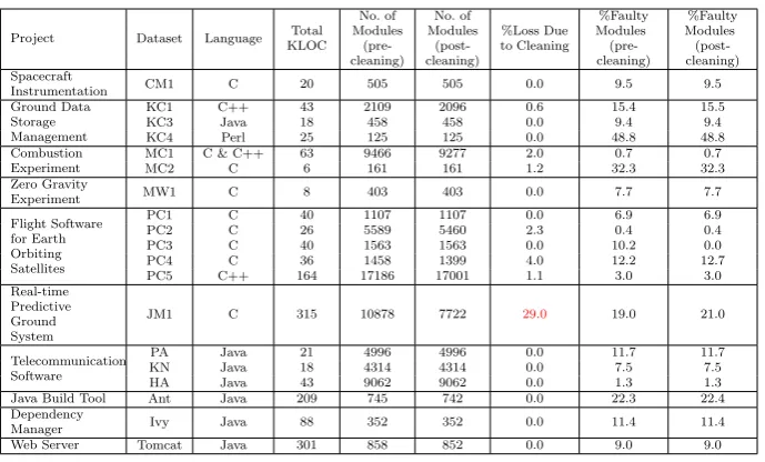
Table 1: Summary Statistics for Data Sets before and after Cleaning
Project Dataset Language Total KLOC No. of Modules (pre-cleaning) No. of Modules (post-cleaning) %Loss Due to Cleaning %Faulty Modules (pre-cleaning) %Faulty Modules (post-cleaning) Spacecraft
Instrumentation CM1 C 20 505 505 0.0 9.5 9.5
Ground Data Storage Management
KC1 C++ 43 2109 2096 0.6 15.4 15.5
KC3 Java 18 458 458 0.0 9.4 9.4
KC4 Perl 25 125 125 0.0 48.8 48.8
Combustion Experiment
MC1 C & C++ 63 9466 9277 2.0 0.7 0.7
MC2 C 6 161 161 1.2 32.3 32.3
Zero Gravity
Experiment MW1 C 8 403 403 0.0 7.7 7.7
Flight Software for Earth Orbiting Satellites
PC1 C 40 1107 1107 0.0 6.9 6.9
PC2 C 26 5589 5460 2.3 0.4 0.4
PC3 C 40 1563 1563 0.0 10.2 0.0
PC4 C 36 1458 1399 4.0 12.2 12.7
PC5 C++ 164 17186 17001 1.1 3.0 3.0
Real-time Predictive Ground System
JM1 C 315 10878 7722 29.0 19.0 21.0
Telecommunication Software
PA Java 21 4996 4996 0.0 11.7 11.7
KN Java 18 4314 4314 0.0 7.5 7.5
HA Java 43 9062 9062 0.0 1.3 1.3
Java Build Tool Ant Java 209 745 742 0.0 22.3 22.4
Dependency
Manager Ivy Java 88 352 352 0.0 11.4 11.4
Web Server Tomcat Java 301 858 852 0.0 9.0 9.0
3.2 Data Sets
We used the NASA data sets first published on the now defunct MDP website8. This repository consists of 13 data sets from a range of NASA projects. In this study we use 12 of the 13 NASA data sets. JM1 was not used because during cleaning, 29% of data was removed suggesting that the quality of the data may have been poor. We extended our previous analysis (Bowes et al. 2015) by using 6 additional data sets, 3 open source and 3 commercial. All 3 open source data sets are at class-level. The commercial data sets are all in the telecommunication domain and are at method level. A summary of each dataset can be found in Table
1.
The data quality of the original NASA MDP data sets can be improved ( Boet-ticher 2006; Gray et al. 2012; Shepperd et al. 2013). Gray et al. (2012); Gray
(2013);Shepperd et al.(2013) describe techniques for cleaning the data. Shepperd has provided a ‘cleaned’ version of the MDP data sets9, however full traceability back to the original items is not provided. Consequently we did not use Shepperd’s cleaned NASA data sets. Instead we cleaned the NASA data sets ourselves. We carried out the following data cleaning stages described by Gray et al. (2012): Each independent variable was tested to see if all values were the same, if they were, this variable was removed because they contained no information which al-lows us to discriminate defective items from non defective items. The correlation for all combinations of two independent variables was found, if the correlation was 1 the second variable was removed. Where the dataset contained the vari-able ‘DECISION DENSITY’ any item with a value of ‘na’ was converted to 0.
8 http://mdp.ivv.nasa.gov– unfortunately now not accessible
The ‘DECISION DENSITY’ was also set to 0 if ‘CONDITION COUNT’=0 and ‘DECISION COUNT’=0. Items were removed if:
1. HALSTEAD LENGTH!= NUM OPERANDS+NUM OPERATORS 2. CYCLOMATIC COMPLEXITY>1+NUM OPERATORS
3. CALL PAIRS>NUM OPERATORS
Our method for cleaning the NASA data also differs from Shepperd et al.
(2013) because we do not remove items where the executable lines of code is zero. We did not do this because we have not been able to determine how the NASA metrics were computed and it is possible to have zero executable lines in Java interfaces. We performed the same cleaning to our commercial data sets. We performed cleaning of the open source data sets for which we defined a similar set of rules as described above, for data at a class level. Particularly, we removed items if:
1. AVERAGE CYCLOMATIC COMPLEXITY>
MAXIMAL CYCLOMATIC COMPLEXITY 2. NUMBER OF COMMENTS>LINES OF CODE
3. PUBLIC METODS COUNT>CLASS METHODS COUNT
3.3 Experimental Set-Up
The following experiment was repeated 100 times. Experiments are more com-monly repeated 10 times. We chose 100 repeats because Mende (2011) reports that using 10 experiment repeats results in an unreliable final performance figure. Each dataset was split into 10 stratified folds. Each fold was held out in turn to form a test set and the other folds were combined and randomised (to reduce ordering effects) to produce the training set. Such stratified cross validation en-sures that there are instances of the defective class in each test set, so reduces the likelihood of classification uncertainty. Re-balancing of the training set is some-times carried out to provide the classifier with a more representative sample of the infrequent defective instances. Re-balancing was not carried out because not all classifiers benefit from this step. For each training/testing pair four different classi-fiers were trained using the same training set. Where appropriate a grid search was performed to identify optimal meta-parameters for each classifier on the training set. The model built by each classifier was used to classify the test set.
To collect the data showing individual predictions made by individual classifiers the RowID, DataSet, runid, foldid and classified label (defective or not defective) was recorded for each item in the test set for each classifier and for each cross validation run.
were then categorised by the original label for each item so that we can see the difference between how the models had classified the defective and non defective items.
Table 2: Confusion Matrix
Predicted defective Predicted defect free Observed
defective
True Positive (TP)
False Negative (FN) Observed
defect free
False Positive (FP)
True Negative (TN)
The confusion matrix is in many ways analogous to residuals for regression models. It forms the fundamental basis from which almost all other performance statistics are derived .
Table 3: Composite Performance Measures
Construct Defined as Description
Recall
pd (probability of detection) Sensitivity
True positive rate
T P/(T P+F N) Proportion of defective units correctly classified
Precision T P/(T P+F P) Proportion of units correctly predicted as defective
pf (probability of false alarm)
False positive rate F P/(F P+T N)
Proportion of non-defective units incor-rectly classified
Specificity
True negative rate T N/(T N+F P) Proportion of correctly classified non de-fective units
F-measure 2·Recall·P recision Recall+P recision
Most commonly defined as the harmonic mean of precision and recall
Accuracy (T N+(T NF N++T PF P)+T P) Proportion of correctly classified units
Matthews Correlation Coeffi-cient
T P×T N−F P×F N √
(T P+F P)(T P+F N)(T N+F P)(T N+F N)
Combines all quadrants of the binary confusion matrix to produce a value in the range -1 to +1 with 0 indicating ran-dom correlation between the prediction and the recorded results. MCC can be tested for statistical significance, with
χ2=N·M CC2whereNis the total number of instances.
4 Results
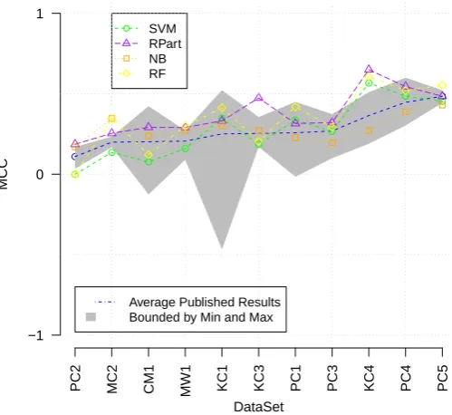
We aim to investigate variation in the individual defects and prediction consis-tency produced by the four classifiers. To ensure the defects that we analyse are reliable we first checked that our models were performing satisfactorily.To do this we built prediction models using the NASA data sets. Figure 1 compares the MCC performance of our models against 600 defect prediction performances re-ported in published studies using these NASA data sets Hall et al.(2012)10. We re-engineered MCC from the performance figures reported in these previous stud-ies using DConfusion. This is a tool we developed for transforming a variety of reported predictive performance measures back to a confusion matrix. DConfusion
[image:11.595.74.418.283.458.2]SVM RPart NB RF
Average Published Results Bounded by Min and Max
PC2 MC2 CM1 MW1 KC1 KC3 PC1 PC3 KC4 PC4 PC5
−1 0 1
DataSet
[image:12.595.111.361.127.356.2]MCC
Fig. 1: Our Results Compared to Results Published by other Studies.
is described in (Bowes et al. 2013). Figure 1shows that the performances of our four classifiers are generally in keeping with those reported by others. Figure 1
confirms that some data sets are notoriously difficult to predict. For example few performances for PC2 are better than random. Whereas very good predictive per-formances are generally reported for PC5 and KC4. The RPart and Na¨ıve Bayes classifiers did not perform as well on the NASA data sets as on our commercial data sets (as shown in Table4). However, all our commercial data sets are highly imbalanced, where learning from a small set of defective items becomes more dif-ficult, so this imbalance may explain the difference in the way these two classifiers perform. Similarly the SVM classifier performs better on the open source data sets than it does on the NASA data sets. The SVM classifier seems to perform particularly poorly when used on extremely imbalanced data sets (especially the case when data sets have less than 10% faulty items).
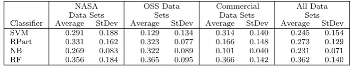
We investigated classifier performance variation across all the data sets. Table
KC4 and KN, but not on the Ivy data set11. Whereas Table 5shows much lower performance figures for Na¨ıve Bayes when used only on the KC4 data set.
Table 4: MCC Performance all Data Sets by Classifier
NASA Data Sets
OSS Data Sets
Commercial Data Sets
All Data Sets
Classifier Average StDev Average StDev Average StDev Average StDev
SVM 0.291 0.188 0.129 0.134 0.314 0.140 0.245 0.154
RPart 0.331 0.162 0.323 0.077 0.166 0.148 0.273 0.129
NB 0.269 0.083 0.322 0.089 0.101 0.040 0.231 0.071
RF 0.356 0.184 0.365 0.095 0.366 0.142 0.362 0.140
Table 5: Performance Measures for KC4, KN and Ivy
KC4 KN Ivy
Classifier MCC F-Measure MCC F-Measure MCC F-Measure
SVM 0.567 0.795 0.400 0.404 0.141 0.167
RPart 0.650 0.825 0.276 0.218 0.244 0.324
NB 0.272 0.419 0.098 0.170 0.295 0.375
RF 0.607 0.809 0.397 0.378 0.310 0.316
Having established that our models were performing acceptably we next wanted to identify the particular defects that each of our four classifiers predicts so that we could identify variations in the defects predicted by each. We needed to be able to label each module as either containing a predicted defect (or not) by each classifier. As we used 100 repeated 10-fold cross validation experiments, we needed to decide on a prediction threshold at which we would label a module as either predicted defective (or not) by each classifier, i.e. how many of these 100 runs must have predicted that a module was defective before we labelled it as such. We analysed the labels that each classifier assigned to each module for each of the 100 runs. There was a surprising amount of prediction ‘flipping’ between runs. On some runs a module was labelled as defective and other runs not. There was variation in the level of prediction flipping amongst the classifiers. Table7 shows the overall label ‘flipping’ between the classifiers.
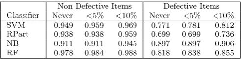
Table 6divides predictions between the actual defective and non-defective la-bels (i.e. the known lala-bels for each module) for each of our data set category, namely NASA, commercial (Comm.), and open source data set (OSS), respec-tively. For each of these two categories, Table6shows three levels of label flipping: never, 5% and 10%. For example, a value of defective items flippingN ever= 0.717 would indicate that 71.7% of defective items never flipped, a value of defective items flipping<5% = 0.746 would indicate that 74.6% of defective items flipped less than 5% of the time. Table 7 suggests that non defective items had a more stable prediction than defective items across all data sets. Although Table7shows the average numbers of prediction flipping across all data sets, this statement is
Table 6: Frequency of all Items Flipping Across Different Data Set Categories
Non Defective Items Defective Items
Classifier Never <5% <10% Never <5% <10%
NASA
SVM 0.983 0.985 0.991 0.717 0.746 0.839
RPart 0.972 0.972 0.983 0.626 0.626 0.736
NB 0.974 0.974 0.987 0.943 0.943 0.971
RF 0.988 0.991 0.993 0.748 0.807 0.859
Comm.
SVM 0.959 0.967 0.974 0.797 0.797 0.797
RPart 0.992 0.992 0.995 0.901 0.901 0.901
NB 0.805 0.805 0.879 0.823 0.823 0.823
RF 0.989 0.992 0.995 0.897 0.897 0.897
OSS
SVM 0.904 0.925 0.942 0.799 0.799 0.799
RPart 0.850 0.850 0.899 0.570 0.570 0.570
NB 0.953 0.953 0.971 0.924 0.924 0.924
[image:14.595.122.368.280.340.2]RF 0.958 0.970 0.975 0.809 0.809 0.809
Table 7: Frequency of all Items Flipping in all Data Sets
Non Defective Items Defective Items
Classifier Never <5% <10% Never <5% <10%
SVM 0.949 0.959 0.969 0.771 0.781 0.812
RPart 0.938 0.938 0.959 0.699 0.699 0.736
NB 0.911 0.911 0.945 0.897 0.897 0.906
RF 0.978 0.984 0.988 0.818 0.838 0.855
valid for all of our data set categories as shown in Table 6. This is probably be-cause of the imbalance of data. Since there is more non-defective items to learn from, predictors could be better trained to predict them, and hence flip less. Al-though the average numbers do not indicate much flipping between modules being predicted as defective or non defective, these tables show data sets together and so the low flipping in large data sets masks the flipping that occurs in individual data sets.
Table 8 shows the label flipping variations during the 100 runs between data sets12. For some data sets using particular classifiers results in a high level of flipping (prediction uncertainty). For example, Table 8 shows that using Na¨ıve Bayes on KN results in prediction uncertainty, with 73% of the predictions for known defective modules flipping at least once between being predicted defective to predicted non defective between runs. Table8also shows the prediction uncertainty of using SVM on the KC4 data set with only 26% of known defective modules being consistently predicted as defective or not defective across all cross validation runs. Figure 2 shows the flipping for SVM on KC4 in more detail13. As a result of analysing these labelling variations between runs, we decided to label a module as having been predicted as either defective or not defective if it had been predicted as such on more than 50 runs. Using a threshold of 50 is the equivalent of choosing the label based on the balance of probability.
12 Label flipping tables for all data sets are available from https://sag.cs.herts.ac.uk/
?page_id=235.
1.0
1.4
1.8
●
●
FN TP
FP TN
1 Non Defective
2 Defective
SVM
1.0
1.4
1.8
●
●
FN TP
FP TN
1 Non Defective
2 Defective
RPart
1.0
1.4
1.8
● ●
FN TP
FP TN
1 Non Defective
2 Defective
NaiveBayes
1.0
1.4
1.8
●
●
FN TP
FP TN
1 Non Defective
2 Defective
[image:15.595.93.392.83.280.2]RandomForest
Fig. 2: Violin Plot of Frequency of Flipping for KC4 Data Set
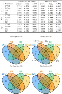
[image:15.595.121.367.319.563.2]Table 8: Frequency of Flipping for Three Different Data Sets
Non defective items Defective Items
Classifier Never <5% <10% Never <5% <10%
K
C4
SVM 0.719 0.734 0.828 0.262 0.311 0.443
RPart 0.984 0.984 1.000 0.902 0.902 0.984
NB 0.938 0.938 0.984 0.885 0.885 0.934
RF 0.906 0.938 0.953 0.803 0.820 0.918
KN
SVM 0.955 0.964 0.971 0.786 0.817 0.854
RPart 0.993 0.993 0.997 0.888 0.888 0.929
NB 0.491 0.491 0.675 0.571 0.571 0.730
RF 0.988 0.991 0.994 0.919 0.922 0.957
Ivy
SVM 0.913 0.949 0.962 0.850 0.850 0.875
RPart 0.837 0.837 0.881 0.625 0.625 0.700
NB 0.933 0.933 0.952 0.950 0.950 1.000
RF 0.955 0.974 0.981 0.900 0.925 0.950
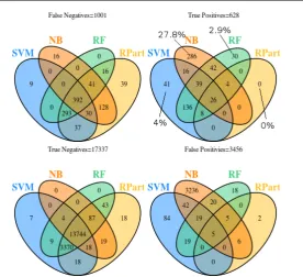
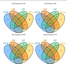
Fig. 4: Sensitivity Analysis for all Open Source Data Sets using Different Classi-fiers. n= 1663 p= 283
Fig. 5: Sensitivity Analysis for all Commercial Data Sets using Different Classifiers. n= 17344 p= 1027
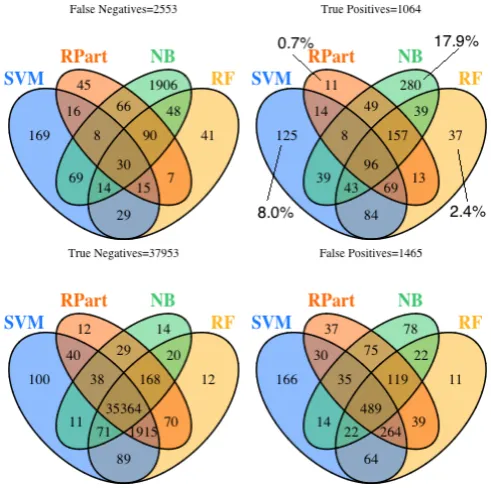
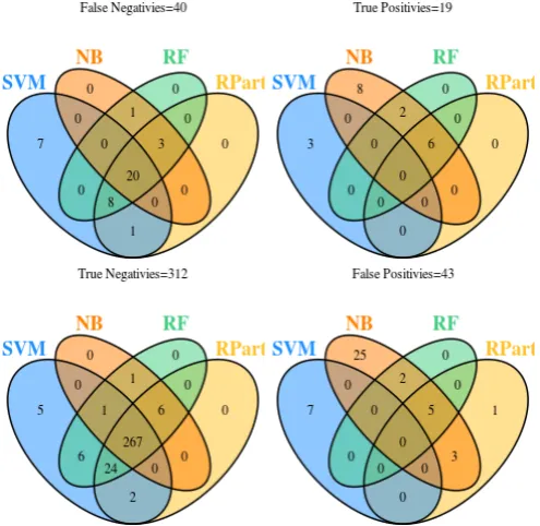
and variation in the actual modules predicted as either defective or not defective by each classifier. Figure3 shows that 96 out of 1568 defective modules are cor-rectly predicted as defective by all four classifiers (only 6.1%). Very many more modules are correctly identified as defective by individual classifiers. For example Na¨ıve Bayes is the only classifier to correctly find 280 (17.9%) defective modules and SVM is the only classifier to correctly locate 125 (8.0%) defective modules (though such predictive performance must always be weighed against false posi-tive predictions). Our results suggest that using only a Random Forest classifier would fail to predict many (526 (34%)) defective modules. Observing Figure4and
5we came to similar conclusions. In the case of the open source data sets, 55 out of 283 (19.4%) unique defects were identified by either Na¨ıve Bayes or SVM. Many more unique defects were found by individual classifiers in the commercial data sets, precisely 357 out of 1027 (34.8%).
There is much more agreement between classifiers about non-defective modules. In the true negative quadrant Figure3shows that all four classifiers agree on 35364 (93.1%) out of 37987 true negative NASA modules. Though again, individual non defective modules are located by specific classifiers. For example, Figure 3
Fig. 6: Sensitivity Analysis for KC4 using Different Classifiers. n= 64 p= 61
[image:18.595.122.370.375.616.2]Fig. 8: KN Sensitivity Analysis using Different Classifiers. n= 3992 p= 322
KC4 data set14. KC4 is an interesting data set. It is unusually balanced between defective and non-defective modules (64 v 61). It is also a small data set (only 125 modules). Figure6shows that for KC4 Na¨ıve Bayes behaves differently compared to how it behaves for the other data sets. In particular for KC4 Na¨ıve Bayes is much less optimistic (i.e. it predicts only 17 out of 125 modules as being defective) in its predictions than it is for the other data sets. RPart was more conservative when predicting defective items than non defective ones. For example, in the KN data set RPart is the only classifier to find 17 (5.3%) unique non-defective items as shown on Figure8.
5 Discussion
Our results suggest that there is uncertainty in the predictions made by classifiers. We have demonstrated that there is a surprising level of prediction flipping be-tween cross validation runs by classifiers. This level of uncertainty is not usually observable as studies normally only publish average final prediction figures. Few studies concern themselves with the results of individual cross validation runs.
Elish and Elish (2008) is a notable exception to this, where the mean and the standard deviation of the performance values across all runs are reported. Few studies run experiments 100 times. More commonly experiments are run only 10 times (e.g.Lessmann et al. 2008;Menzies et al. 2007). This means that the level of
prediction flipping between runs is likely to be artificially reduced. We suspect that prediction flipping by a classifier for a data set is caused by the random generation of the folds. The items making up the individual folds determine the composition of the training data and the model that is built. The larger the data set the less prediction flipping occurs. This is likely to be because larger data sets may have training data that is more consistent with the entire data set. Some classifiers are more sensitive to the composition of the training set than other classifiers. SVM is particularly sensitive for KC4 where 26% of non defective items flip at least once and 44% of defective items flip. Although SVM performs well (MCC = 0.567), the items it predicts as being defective are not consistent across different cross validation runs. Future research is needed to use our results on flipping to iden-tify the threshold at which overall defective or not defective predictions should be determined.
The level of uncertainty among classifiers may be valuable for practitioners in different domains of defect predictions. For instance, where stability of prediction plays a significant role our results suggest that on average Na¨ıve Bayes would be the most suitable selection. On the other hand, learners such as RPart may be avoided in applications where higher prediction consistency is needed. The reasons for this prediction inconsistency are yet to be established. More classifiers with different properties should also be investigated to establish the extent of uncertainty in predictions.
Other large scale studies comparing the performance of defect prediction mod-els show that there is no significant difference between classifiers (Arisholm et al. 2010; Lessmann et al. 2008). Our overall MCC values for the four classifiers we investigate also suggest performance similarity. Our results show that specific clas-sifiers are sensitive to data set and that classifier performance varies according to data set. For example, our SVM model performs poorly on Ivy but performs much better on KC4. Other studies have also reported sensitivity to data set (e.g. Less-mann et al. 2008).
Similarly to Panichella et al.(2014), our results also suggest that overall per-formance figures hide a variety of differences in the defects that each classifier predicts. While overall performance figures between classifiers are similar, very different subsets of defects are actually predicted by different classifiers. So it would be wrong to conclude that, given overall performance values for classifiers are similar, it does not matter which classifier is used. Very different defects are predicted by different classifiers. This is probably not surprising given that the four classifiers we investigate approach the prediction task using very different techniques. Future work is needed to investigate whether there is any similarity in the characteristics of the set of defects that each classifier predicts. Currently it is not known whether particular classifiers specialise in predicting particular types of defect.
defects that individual classifiers predict. Again, future work is needed to establish a decision making approach for ensembles that will exploit our findings.
6 Threats to Validity
Although we implemented what could be regarded as current best practice in classifier-based model building, there are many different ways in which a classifier may be built. There are also many different ways in which the data used can be pre-processed. All of these factors are likely to impact on predictive performance. As Lessmann et al. (2008) say classification is only a single step within a mul-tistage data mining process (Fayyad et al. 1996). Especially, data preprocessing or engineering activities such as the removal of non informative features or the discretisation of continuous attributes may improve the performance of some clas-sifiers (see, e.g.,Dougherty et al. 1995; Hall and Holmes 2003). Such techniques have an undisputed value. Despite the likely advantages of implementing these many additional techniques, as Lessmann et al. we implemented only a basic set of these techniques. Our reason for this decision was the same as Lessmann et al.
...computationally infeasible when considering a large number of classifiers at the same time. The experiments we report here each took several days of processing time. We did implement a set of techniques that are commonly used in defect prediction of which there is evidence they improve predictive performance. We went further in some of the techniques we implemented e.g. running our experi-ments 100 times rather than the 10 times that studies normally do. However we did not implement a technique to address data imbalance (e.g. SMOTE). This was because data imbalance does not affect all classifiers equally. We implemented only partial feature reduction. The impact of the model building and data pre-processing approaches we used are not likely to significantly affect the results we report. In addition the range of approaches we used are comparable to current defect prediction studies.
Our studies are also limited in that we only investigated four classifiers. It may be that there is less variation in the defect subsets detected by classifiers that we did not investigate. We believe this to be unlikely, as the four classifiers we chose are representative of discrete groupings of classifiers in terms of the prediction approaches used. However future work will have to determine whether additional classifiers behave as we report these four classifiers to. We also used a limited number of data sets in our study. Again, it is possible that other data sets behave differently. We believe this will not be the case, as the 18 data sets we investigated were wide ranging in their features and produced a variety of results in our investigation.
of classification algorithms in the context of defect prediction and proposed other performance metrics that are independent from the specific (and also implicit) cut-off points used by different classifiers. Future work includes consideration of the different cut-off points to the individual performances of the four classifiers used in this paper.
7 Conclusion
We report a surprising amount of prediction variation within experimental runs. We repeated our cross validation runs 100 times. Between these runs we found a great deal of inconsistency in whether a module was predicted as defective or not by the same model. This finding has important implications for defect prediction as many studies only repeat experiments 10 times. This means that the reliability of some previous results may be compromised. In addition the prediction flipping that we report has implications for practitioners. Although practitioners may be happy with the overall predictive performance of a given model, they may not be so happy that the model predicts different modules as defective depending on the training of the model.
Performance measures can make it seem that defect prediction models are performing similarly. However, even where similar performance figures are pro-duced, different defects are identified by different classifiers. This has important implications for defect prediction. First, assessing predictive performance using conventional measures such as f-measure, precision or recall gives only a basic pic-ture of the performance of models (Fenton and Neil 1999). Second, models built using only one classifier are not likely to comprehensively detect defects. Ensem-bles of classifiers need to be used. Third, current approaches to ensemEnsem-bles need to be re-considered. In particular the popular ‘majority’ voting decision approach used by ensembles will miss the sizeable sub-sets of defects that single classifiers correctly predict. Ensemble decision-making strategies need to be enhanced to ac-count for the success of individual classifiers in finding specific sets of defects. As Panichella et al. suggested, techniques such as “local prediction” may be suitable for within-project defect prediction as well.
The feature selection techniques for each classifier could also be explored in future. Since different classifiers find different sub-set of defects it is reasonable to explore whether some particular features better suit specific classifiers. Perhaps some classifiers work better when combined with specific sub-sets of features.
We suggest new ways of building enhanced defect prediction models and oppor-tunities for effectively evaluating the performance of those models in within-project studies. These opportunities could provide future researchers with the tools with which to break through the performance ceiling currently being experienced in defect prediction.
References
Arisholm E, Briand LC, Fuglerud M (2007) Data mining techniques for building fault-proneness models in telecom java software. In: Software Reliability, 2007. ISSRE ’07. The 18th IEEE International Symposium on, pp 215 –224
Arisholm E, Briand LC, Johannessen EB (2010) A systematic and comprehensive investigation of methods to build and evaluate fault prediction models. Journal of Systems and Software 83(1):2–17
Bell R, Ostrand T, Weyuker E (2006) Looking for bugs in all the right places. In: Proceedings of the 2006 international symposium on Software testing and analysis, ACM, pp 61–72 Bibi S, Tsoumakas G, Stamelos I, Vlahvas I (2006) Software defect prediction using regression
via classification. In: Computer Systems and Applications. IEEE International Conference on.
Bird C, Bachmann A, Aune E, Duffy J, Bernstein A, Filkov V, Devanbu P (2009a) Fair and balanced?: bias in bug-fix datasets. In: Proceedings of the the 7th joint meeting of the European software engineering conference and the ACM SIGSOFT symposium on The foundations of software engineering, ACM, New York, NY, USA, ESEC/FSE ’09, pp 121– 130
Bird C, Nagappan N, Gall H, Murphy B, Devanbu P (2009b) Putting it all together: Using socio-technical networks to predict failures. In: 20th International Symposium on Software Reliability Engineering, IEEE, pp 109–119
Boetticher G (2006) Advanced machine learner applications in software engineering, Idea Group Publishing, Hershey, PA, USA, chap Improving credibility of machine learner mod-els in software engineering, pp 52 – 72
Bowes D, Hall T, Gray D (2013) DConfusion: a technique to allow cross study performance evaluation of fault prediction studies. Automated Software Engineering pp 1–27, DOI 10.1007/s10515-013-0129-8, URLhttp://dx.doi.org/10.1007/s10515-013-0129-8 Bowes D, Hall T, Petri´c J (2015) Different classifiers find different defects although with
differ-ent level of consistency. In: Proceedings of the 11th International Conference on Predictive Models and Data Analytics in Software Engineering, PROMISE ’15, pp 3:1–3:10, DOI 10.1145/2810146.2810149, URLhttp://doi.acm.org/10.1145/2810146.2810149 Briand L, Melo W, Wust J (2002) Assessing the applicability of fault-proneness models across
object-oriented software projects. Software Engineering, IEEE Transactions on 28(7):706 – 720
Catal C, Diri B (2009) A systematic review of software fault prediction studies. Expert Systems with Applications 36(4):7346–7354
Chawla NV, Japkowicz N, Kotcz A (2004) Editorial: special issue on learning from imbalanced data sets. SIGKDD Explorations 6(1):1–6
Chen H, Yao X (2009) Regularized negative correlation learning for neural network ensembles. Neural Networks, IEEE Transactions on 20(12):1962–1979
D’Ambros M, Lanza M, Robbes R (2009) On the relationship between change coupling and software defects. In: Reverse Engineering, 2009. WCRE ’09. 16th Working Conference on, pp 135 –144
Dougherty J, Kohavi R, Sahami M (1995) Supervised and unsupervised discretization of con-tinuous features. In: ICML, pp 194–202
Elish K, Elish M (2008) Predicting defect-prone software modules using support vector ma-chines. Journal of Systems and Software 81(5):649–660
Fayyad U, Piatetsky-Shapiro G, Smyth P (1996) From data mining to knowledge discovery in databases. AI magazine 17(3):37
Fenton N, Neil M (1999) A critique of software defect prediction models. Software Engineering, IEEE Transactions on 25(5):675 –689
Gray D (2013) Software defect prediction using static code metrics : Formulating a methodol-ogy. PhD thesis, Computer Science, University of Hertfordshire
Gray D, Bowes D, Davey N, Sun Y, Christianson B (2012) Reflections on the nasa mdp data sets. Software, IET 6(6):549 –558
Hall MA, Holmes G (2003) Benchmarking attribute selection techniques for discrete class data mining. Knowledge and Data Engineering, IEEE Transactions on 15(6):1437–1447 Hall T, Beecham S, Bowes D, Gray D, Counsell S (2012) A systematic literature review on fault
Jiang Y, Lin J, Cukic B, Menzies T (2009) Variance analysis in software fault prediction models. In: SSRE 2009, 20th International Symposium on Software Reliability Engineering, IEEE Computer Society, Mysuru, Karnataka, India, 16-19 November 2009, pp 99–108
Khoshgoftaar T, Yuan X, Allen E, Jones W, Hudepohl J (2002) Uncertain classification of fault-prone software modules. Empirical Software Engineering 7(4):297–318
Khoshgoftaar TM, Gao K, Seliya N (2010) Attribute selection and imbalanced data: Problems in software defect prediction. In: Tools with Artificial Intelligence (ICTAI), 2010 22nd IEEE International Conference on, vol 1, pp 137–144
Kim S, Zhang H, Wu R, Gong L (2011) Dealing with noise in defect prediction. In: Proceedings of the 33rd International Conference on Software Engineering, ACM, New York, NY, USA, ICSE ’11, pp 481–490
Kutlubay O, Turhan B, Bener A (2007) A two-step model for defect density estimation. In: Software Engineering and Advanced Applications, 2007. 33rd EUROMICRO Conference on, pp 322 –332
Lessmann S, Baesens B, Mues C, Pietsch S (2008) Benchmarking classification models for soft-ware defect prediction: A proposed framework and novel findings. Softsoft-ware Engineering, IEEE Transactions on 34(4):485 –496
Liebchen G, Shepperd M (2008) Data sets and data quality in software engineering. In: Pro-ceedings of the 4th international workshop on Predictor models in software engineering, ACM, pp 39–44
M D’Ambros ML, Robbes R (2012) Evaluating defect prediction approaches: a benchmark and an extensive comparison. Empirical Software Engineering 17(4):531–577
Mende T (2011) On the evaluation of defect prediction models. In: The 15th CREST Open Workshop
Mende T, Koschke R (2010) Effort-aware defect prediction models. In: Software Maintenance and Reengineering (CSMR), 2010 14th European Conference on, pp 107–116
Menzies T, Greenwald J, Frank A (2007) Data mining static code attributes to learn defect predictors. Software Engineering, IEEE Transactions on 33(1):2 –13
Menzies T, Turhan B, Bener A, Gay G, Cukic B, Jiang Y (2008) Implications of ceiling effects in defect predictors. In: Proceedings of the 4th international workshop on Predictor models in software engineering, pp 47–54
Menzies T, Caglayan B, He Z, Kocaguneli E, Krall J, Peters F, Turhan B (2012) The promise repository of empirical software engineering data. URLhttp://promisedata.googlecode. com
Minku LL, Yao X (2012) Ensembles and locality: Insight on improving software effort estima-tion. Information and Software Technology
Minku LL, Yao X (2013) Software effort estimation as a multi-objective learning problem. ACM Transactions on Software Engineering and Methodology, to appear
Mısırlı AT, Bener AB, Turhan B (2011) An industrial case study of classifier ensembles for locating software defects. Software Quality Journal 19(3):515–536
Mizuno O, Kikuno T (2007) Training on errors experiment to detect fault-prone software modules by spam filter. In: Proceedings of the the 6th joint meeting of the European software engineering conference and the ACM SIGSOFT symposium on The foundations of software engineering, ACM, New York, NY, USA, ESEC-FSE ’07, pp 405–414 Mizuno O, Ikami S, Nakaichi S, Kikuno T (2007) Spam filter based approach for finding
fault-prone software modules. In: Mining Software Repositories, 2007. ICSE Workshops MSR ’07. Fourth International Workshop on, p 4
Myrtveit I, Stensrud E, Shepperd M (2005) Reliability and validity in comparative studies of software prediction models. IEEE Transactions on Software Engineering pp 380–391 Nagappan N, Zeller A, Zimmermann T, Herzig K, Murphy B (2010) Change bursts as defect
predictors. In: Software Reliability Engineering, 2010 IEEE 21st International Symposium on, pp 309–318
Ostrand T, Weyuker E, Bell R (2010) Programmer-based fault prediction. In: Proceedings of the 6th International Conference on Predictive Models in Software Engineering, ACM, pp 1–10
Seiffert C, Khoshgoftaar TM, Hulse JV (2009) Improving software-quality predictions with data sampling and boosting. IEEE Transactions on Systems, Man, and Cybernetics, Part A 39(6):1283–1294
Shepperd M, Kadoda G (2001) Comparing software prediction techniques using simulation. Software Engineering, IEEE Transactions on 27(11):1014 –1022
Shepperd M, Song Q, Sun Z, Mair C (2013) Data quality: Some comments on the nasa software defect datasets. Software Engineering, IEEE Transactions on 39(9):1208–1215, DOI 10. 1109/TSE.2013.11
Shin Y, Bell RM, Ostrand TJ, Weyuker EJ (2009) Does calling structure information improve the accuracy of fault prediction? In: Godfrey MW, Whitehead J (eds) Proceedings of the 6th International Working Conference on Mining Software Repositories, IEEE, pp 61–70 Shivaji S, Whitehead EJ, Akella R, Sunghun K (2009) Reducing features to improve bug
predic-tion. In: Automated Software Engineering, 2009. ASE ’09. 24th IEEE/ACM International Conference on, pp 600–604
Soares C, Brazdil PB, Kuba P (2004) A meta-learning method to select the kernel width in support vector regression. Machine learning 54(3):195–209
Sun Z, Song Q, Zhu X (2012) Using coding-based ensemble learning to improve software defect prediction. Systems, Man, and Cybernetics, Part C: Applications and Reviews, IEEE Transactions on 42(6):1806–1817, DOI 10.1109/TSMCC.2012.2226152
Visa S, Ralescu A (2004) Fuzzy classifiers for imbalanced, complex classes of varying size. In: Information Processing and Management of Uncertainty in Knowledge-Based Systems, pp 393–400
Witten I, Frank E (2005) Data Mining: Practical machine learning tools and techniques. Mor-gan Kaufmann
Wolpert DH (1992) Stacked generalization. Neural Networks 5(2):241 – 259, DOI http://dx. doi.org/10.1016/S0893-6080(05)80023-1, URL http://www.sciencedirect.com/science/ article/pii/S0893608005800231
Zhang H (2009) An investigation of the relationships between lines of code and defects. In: Software Maintenance, 2009. ICSM 2009. IEEE International Conference on, pp 274–283 Zhou Y, Xu B, Leung H (2010) On the ability of complexity metrics to predict fault-prone