Artificial Bee Colony Algorithm with Adaptive Explorations and Exploitations: A Novel Approach for Continuous Optimization

Artificial Bee Colony Algorithm with Adaptive

Explorations and Exploitations: A Novel Approach for

Continuous Optimization

Mohammad Shafiul Alam

Department of Computer Science and Engineering Ahsanullah University of Science and Technology Dhaka-1208, Bangladesh

Md. Monirul Islam

Department of Computer Science and Engineering Bangladesh University of Engineering and Technology

Dhaka-1000, Bangladesh

Kazuyuki Murase

Department of Human and Artificial Intelligence Systems

University of Fukui Fukui 910-8507, Japan

ABSTRACT

A proper balance between global explorations and local exploitations is often considered necessary for complex, high dimensional optimization problems to avoid local optima and to find a good near optimum solution with sufficient convergence speed. This paper introduces Artificial Bee Colony algorithm with Adaptive eXplorations and eXploitations (ABC-AX2), a novel algorithm that improves over the basic Artificial Bee Colony (ABC) algorithm. ABC-AX2 augments each candidate solution with three control parameters that control the perturbation rate, magnitude of perturbations and proportion of explorative and exploitative perturbations. Together, all the control parameters try to adapt the degree of global explorations and local exploitations around each candidate solution by affecting how new trial solutions are produced from the existing ones. The control parameters are automatically adapted at the individual solution level, separately for each candidate solution. ABC-AX2 is tested on a number of benchmark problems of continuous optimization and compared with the basic ABC algorithm and several other recent variants of ABC algorithm. Results show that the performance of ABC-AX2 is often better than most other algorithms in comparison, in terms of both convergence speed and final solution quality.

Keywords

Artificial bee colony algorithm; Exploration and exploitation; Continuous optimization; Meta-heuristic optimization.

1.

INTRODUCTION

The Artificial Bee Colony (ABC) algorithm is a recently introduced [1] swarm intelligence algorithm that tries to mimic the intelligent food foraging behavior of honey bees. Since its advent, the ABC algorithm has been successfully applied to wide and diverse range of problems, such as continuous optimization [2], discrete optimization [3], constrained optimization [4], multi-objective optimization [5], design optimization [6], training neural network [7], design of digital IIR filter [8], PID controller [9], parameterizing of milling processes [10] and so on [11]. ABC is simple in concept, easy to implement and requires fewer control parameters [12]. ABC shows very competitive and often better performance in comparison to many other existing evolutionary and swarm intelligence algorithms [2], such as genetic algorithm (GA), differential evolution (DE) and particle swarm optimization (PSO).

Similar to other population based meta-heuristic algorithms, ABC also has its own challenges and limitations. For example, ABC can prematurely converge to local optima, especially for complex high dimensional multimodal problems [2,13]. Also, the convergence speed of ABC is usually slower than some other meta-heuristic algorithms, such as DE and PSO, especially on unimodal problems [2]. Another problem that may occur with ABC is fitness stagnation [14], where the entire population of solutions stops improving, even without converging to some local optima, because the fitness based selection scheme fails to find new, better trial solutions that can enter the population by replacing the existing solutions. All these problems originate from a lack of balance between global explorations and local exploitations during the optimization procedure. ABC drives its search towards global optimum with two operators — perturbation and selection. The perturbation operation is responsible for explorations by random variations of existing solutions, while the fitness based selection operation performs exploitations of the search regions explored so far. However, both these operations are more aligned towards exploitations than explorations. The perturbation operation of ABC perturbs a single parameter of an existing solution and thus produces the new trial solution in the neighborhood of the original solution, which is exploitative. The selection operation of ABC can accept only the better solutions, which is exploitative too. This paper introduces ABC with Adaptive eXplorations and eXploitations (ABC-AX2), a novel improvement over the basic ABC algorithm that tries to automatically adapt the degree of explorations and exploitations, separately for every candidate solution of the population. ABC AX2 augments each candidate solution xi

with three control parameters– pi, qi and ηi, each of which

affects the perturbation operations on xi to control the degree of explorations and exploitations around xi. The values of pi, qi and ηi are automatically adjusted, cycle (i.e., iteration) by

cycle, using adaptive and self-adaptive techniques to increase the likelihood of producing more effective perturbations on xi.

2.

THE ABC ALGORITHM

Honey bees in nature have to forage over a vast area in search of good sources of nectar. After an initial exploration stage, more bees are employed to collect honey from more profitable food sources whereas fewer bees are assigned to the less worthy sources. After returning the hive, each bee goes to the ‗dance floor‘ and performs a special dance known as the ‗waggle dance‘ to share the information of the food source it has found. The ‗onlooker‘ bees, waiting around the dance floor, observe the waggle dances of the ‗employed‘ bees and pick any of them to follow and collect nectar from the vicinity of its food source. Some scout bees are also assigned for random explorations of the search space to find new food sources. The basic ABC algorithm [1,2] mimics the food foraging behavior of honey bees with the same three groups of bees — employed, onlooker and scout bees. A bee working to forage a particular food source (i.e., candidate solution) and searching only around its vicinity is called an employed bee. Onlooker bees randomly pick and follow any of the employed bees. The probability of picking an employed bee is proportional to the quality of its food source. Scout bees can perform random explorations of the search space to find new food sources. If the employed and onlooker bees, even after limit attempts, fail to find a better food position around a particular food xi, then xi is abandoned and replaced by

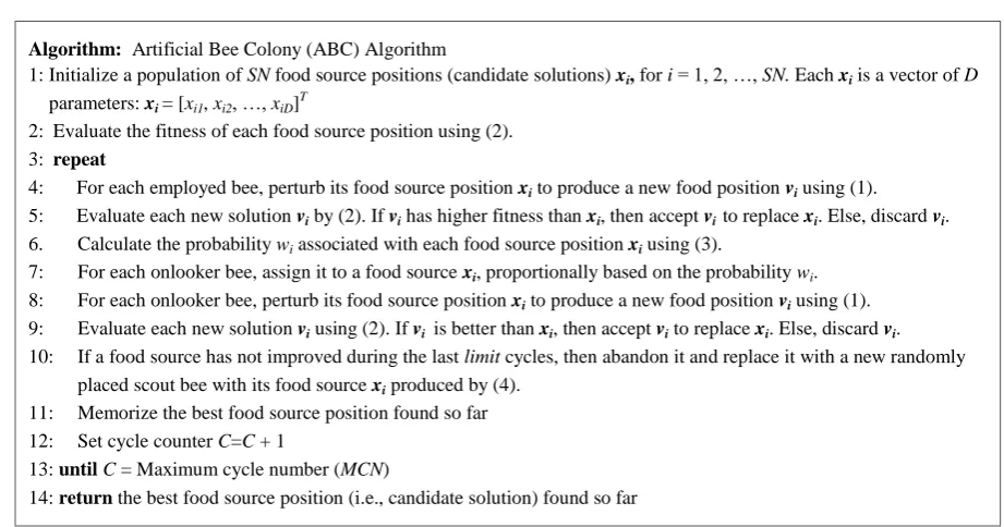
initiating a scout bee and its food source is placed uniformly at random across the search space. In the original implementation of the ABC algorithm, half of the colony is employed bees, the other half is onlooker bees, and scout bees are created on demand only when a food source fails to improve with several attempts. Fig. 1 presents the pseudocode for the basic ABC algorithm. Each cycle (i.e., iteration) of ABC consists of foraging by the employed bees (steps 4–5, Fig. 1), then foraging by the onlookers (steps 7–9), followed by placement of the scout bees (step 10). Each of these stages is described below.

Foraging by employed bees: Suppose, an employed bee is currently positioned at a food source position xi. During this

stage, each employed bee searches in the vicinity of its current position xi to produce new trial food source vi using (1), where j∈ {1, 2, …, D} and k∈ {1, 2, …, SN} are randomly picked indices, D is dimensionality of the problem, SN is the number of food positions and φij is a uniform random value ~ [-1, 1].

vij = xij + φij (xkj – xij) (1)

Thus, the new solution vi is produced from xi by perturbing its

randomly picked j-th parameter and using the information of

xi and another randomly picked solution xk. If vi has better

‗fitness‘ than the old food position xi, then xi is replaced by vi.

For the problem of function optimization, where f is the function to be minimized, ABC computes the ‗fitness‘ of a candidate solution xi using (2).

 

 

 

 

1

; if

0

1

1

otherwise

i i i i fitness

f

f

f



















x

x

x

x

(2)

Foraging by onlooker bees: During this stage, each onlooker bee randomly picks an employed bee to follow and forages only around the vicinity of its food source. The probability wi

that the employed bee with food source xi would be picked by

an onlooker bee is computed using (3), which makes the probability wi to be proportional to fitness(xi).

 

 

1 i i _SN n n fitness x w fitness x  



(3)

Like the employed bees, each onlooker bee also employs (1) to produce trial food source vi in the vicinity of its current

food source position xi. If vi has better fitness than xi, then xi

is replaced by vi. Otherwise, vi is discarded.

Placement of Scout bees: A scout bee is created only when a particular food source xi failed to be improved over the last ‗limit‘ iterations. The bee employed to xi now becomes a

scout bee and its food source is positioned at random across the search space using (4), where j = 1, 2, …, D and [minj, maxj] is the search space along the j-th dimension.

xij = minj + rand (0,1) * (maxj – minj) (4)

3.

EXISTING VARIANTS OF ABC

ALGORITHM

There exist a number of recent studies (e.g., [15]–[24]) that try to alter the explorative and/or exploitative properties of the basic ABC algorithm. For example, ABC with self-adaptive mutation (ABC-SAM) [15] introduces an adaptive mutation scaling factor SFi for every candidate solution xi and tries to

ensure both explorations and exploitations by periodically adjusting the value of SFi using two different distributions —

one explorative and the other exploitative. The SFi values can

candidate solution separately; rather they employ some population-wide global strategy, identically for all candidate solutions, which is significantly improved in the proposed algorithm — ABC-AX2, as described in the following section.

Fig. 1: Algorithm for the basic Artificial Bee Colony (ABC) algorithm

4.

THE PROPOSED ALGORITHM —

ABC-AX

2

ABC-AX2 tries to improve over the basic ABC algorithm by adapting and customizing the degree of explorations and exploitations at the individual solution level, i.e., separately for every candidate solution. ABC-AX2 includes three control parameters – pi, qi and ηiwithin each candidate solution xi.

The control parameter pi controls the proportion of explorative

and exploitative perturbations; qi controls the perturbation rate

to produce vi from xi; ηi=[ηi1, ηi2, …, ηiD] T

is a vector with D

components, each one (say, ηij) of which controls the

distribution of the scaling factor values (i.e., φij values in (1))

during perturbations along the corresponding (i.e., j-th) dimension. Each control parameter is gradually adapted to achieve higher rate of ‗successful‘ perturbations. A perturbation is considered ‗successful‘ only if the new trial solution vi has higher fitness value than the original solution

xi. A detailed description of the role of each control

parameter, how it affects explorations and exploitations in perturbations and how it is gradually adapted by ABC-AX2 are presented in the following paragraphs.

A. Control parameter pi for adaptive proportion of

explorations and exploitations: The basic ABC algorithm

uses the single perturbation scheme (1), with no attempt to differentiate between explorative or exploitative perturbations. In contrast, ABC-AX2 employs two different perturbation schemes — one for explorations, the other for exploitations. Both the perturbation schemes are based on the same expression (1), but they differ in how xi selects itssupporting

candidate solution xk in (1). For explorative perturbations, xk

is picked by three-tier explorative tournament selection (3T-ER-TS), while the exploitative perturbations use two-tier

exploitative tournament selection (2T-ET-TS) procedure. Both the selection procedures are introduced in Fig. 2.

Explorative perturbation:

vij = xij + φij (xkj – xij), where xk ~ 3T-ER-TS(xi) (5)

Exploitative perturbation:

vij = xij + φij (xkj – xij), where xk ~ 2T-ET-TS(xi) (6)

The explorative 3T-ER-TS scheme tries to pick a candidate solution xk that is not only fit, but also dissimilar (from the

current solution xi) and diverse (from the other solutions of

the population). Dissimilarity of xk from xi is measured as

their Euclidean distance (ED), while diversity of xk is

estimated as its ED from the centroid of population of solutions. High dissimilarity of xk from xi ensures a large

|xkj



xij| in (5) to make a large, explorative perturbation on xi,

while the high diversity of xk tries to pull xi away from the

population centroid to promote more diversity and to avoid being trapped around local optima. In contrast, the exploitative 2T-ET-TS scheme tries to pick an xk that is both

fit and has high degree of similarity to xi. This tries to ensure a

small |xkj



xij| in (6) to make small, exploitative steps towards

the better regions of the search space.

But how does ABC-AX2 decide on whether to perform explorative or exploitative perturbation on xi? This is done

probabilistically — the current values of pi and 1–pi denote

the probability of exploitative and explorative perturbations on xi, respectively. The value of pi is automatically adapted

using the incremental learning experience of xi, which

includes the number of successes and failures by explorative and exploitative perturbations on xi during the last τ1 cycles

(learning period). Initially, pi is set to 0.5 for every solution xi,

Algorithm: Artificial Bee Colony (ABC) Algorithm

1: Initialize a population of SN food source positions (candidate solutions) xi, for i = 1, 2, …, SN. Each xi is a vector of D

parameters: xi = [xi1, xi2, …, xiD]T

2: Evaluate the fitness of each food source position using (2).

3: repeat

4: For each employed bee, perturb its food source position xi to produce a new food position vi using (1). 5: Evaluate each new solution vi by (2). If vi has higher fitness than xi, then accept vi to replace xi. Else, discard vi. 6. Calculate the probability wi associated with each food source position xi using (3).

7: For each onlooker bee, assign it to a food source xi, proportionally based on the probability wi.

8: For each onlooker bee, perturb its food source position xi to produce a new food position vi using (1).

9: Evaluate each new solution vi using (2). If vi is better than xi, then accept vi to replace xi. Else, discard vi. 10: If a food source has not improved during the last limit cycles, then abandon it and replace it with a new randomly

placed scout bee with its food source xi produced by (4). 11: Memorize the best food source position found so far 12: Set cycle counter C=C + 1

13: until C = Maximum cycle number (MCN)

which makes exploitative and explorative perturbations equally desired. After the initial learning period of τ1 cycles,

ABC-AX2 starts adjusting the pi value for each xi. To do this,

ABC-AX2 keeps record of the number of successes and failures by exploitative and explorative perturbations on xi

over the last τ1 cycles. Suppose nsERand nfER (nsETand nfET)

are the number of successes and failures, respectively by the explorative (exploitative) perturbations on xi during the last τ1

cycles. Then, success ratios of explorative perturbation (SRER)

and exploitative perturbation (SRET) on xi are computed as: SRER = (nsER) / (nsER + nfER) and SRET = (nsET) / (nsET + nfET).

Now, the adjusted probability of exploitative perturbation on

xi (i.e., the adjusted value of pi) is computed using (7), which

also ensures 0.1 ≤ pi ≤ 0.9 to avoid the complete domination

by either mode of perturbations. Once the value of pi for each

candidate solution xi is computed by ABC-AX2 using (7), it is

kept unchanged for the next τ2 cycles (τ2 <τ1), which allows

some time for the adjusted value of pi to produce both

successes and failures by each type of perturbation. ABC-AX2 regularly adjusts the value of pi for each candidate solution xi

using (7), periodically after each τ2 cycles, using the recorded

values of number of successes and failures by each type of perturbation on xi over the last τ1 cycles. After some initial

experiments, these parameters are set as τ1=50 and τ2=10.

min 0.9, max 0.1, ET

i ER ET SR p SR SR     _  _ _  

  (7)

B. Control parameter qi for self-adaptive

perturbation rate: The basic ABC algorithm perturbs only a single, random parameter of xi using (1). This usually

produces the trial solution vi in the neighbourhood of the

original solution xi, which is exploitative. Perturbing a single

parameter allows search along a single dimension at a time. This may work well for separable problems, but not suitable for non-separable problems where the parameters are not independent. Fig. 3 shows an example using a 2D search space. Allowing perturbation of both the parameters (i.e., xi1

and xi2) canproduce vialong any possible direction from xi.

This is more efficient than perturbing either xi1 or xi2, one at a

time, as is done by the basic ABC algorithm that allows search along axis directions only. In contrast, ABC-AX2 tries to perform search along any possible direction from xi by

maintaining and automatically adapting a control parameter qi,

separately for every candidate solution xi, that controls the

perturbation rate during producing the trial solution vi from xi.

When ABC-AX2 _{wants to perturb a solution x}

i to produce vi,

the value of qi is perturbed first, with probability=u1 using (8),

before perturbing any other parameter of xi. This perturbed

value of qi is inherited by vi, which is henceforth referred as vi.q and is used as the probability of perturbing the parameters

of xi during producing vi from xi. A more appropriate value of vi.q is likely to produce fitter new solutions, which are

supposed to survive better than xi and produce better, newer

solutions and hence, propagate the better value of the perturbation probability. Thus a gradual self-adaptation towards better, more effective qi values takes place, allowing

a self-adaptive and appropriate perturbation rate for the candidate solutions across the population.

  



 

1

rand 0,1 ; if rand 0,1

. otherwise

+

=

i i

min max min

q q q u

q q       v (8)

Here, u1 is the probability that the perturbation probability qi

itself is perturbed before perturbing the parameters of xi. In

ABC-AX2 implementation, these parameters have been set as

u1=0.10, qmax=1.0 and qmin=1/D.

C. Control parameter ηi for self-adaptive

perturbation scaling factors: The basic ABC algorithm

draws the φij values in (1) uniformly at random from [-1, 1],

without any attempt to perform adaptation of the φij values for

more effective perturbations on xi. In contrast, ABC-AX2

produces φij values from a Gaussian distribution with mean=0

and standard deviation=ηij, where ηi=[ηi1, ηi2, …, ηiD]T is a

control parameter vector that is maintained separately for each candidate solution xiand is gradually self-adapted using (9)

and (10). Although this procedure is similar to the self-adaptation strategy adopted in some other previous evolutionary algorithms [25], it has not yet been employed and tested with the ABC algorithm.

for j = 1, 2, …, D

 

 



0,1

0,1



exp

N

j

η

ij



=

η

ij

τ



+τ N

(9) (9)

 

2

if

otherwise

0,1

rand

u











i i i .

η

v η =

η

(10)

Here u2 is the probability that the new trial solution vi gets a

control parameter vi.η that is different from ηi of the original

solution xi. ABC-AX2 uses u2=0.5. The N(0,1) and Nj(0,1) are

random numbers produced from the Normal distribution with mean=0 and standard deviation=1. The subscript j in Nj(0,1)

indicates that the random number is generated anew for each value of j. The τ and τʹ are called learning rates and are set as suggested in [25]. ABC-AX2 maintains a separate ηi for every

solution xi, which enables each xi to customize its own degree

of explorations and exploitations, separately along the D

different axis directions of the search space, using the components of ηi=[ηi1, ηi2, …, ηiD]T. An effective value for vi.η is likely to produce better, fitter new solutions that should

survive better than xi and thus a gradual self-adaptation

towards better, more effective ηi values can take place, cycle

by cycle, across the population.

5.

EXPERIMENTAL STUDIES

To evaluate the performance of ABC-AX2 and to compare it with the basic ABC [2] and some other recent ABC-variants (e.g., [15]–[21]), this paper uses a set of benchmark problems which has 30 standard functions, including 18 scalable high dimensional functions with dimensionality D=30, 60, as well as 12 low dimensional multimodal functions with D ≤ 10. The suite contains both unimodal (i.e., f1–f9) and multimodal (i.e., f10–f30), separable (e.g., f1, f3, f8) and non-separable (e.g., f2, f4, f5), high (i.e., f1–f18) and low (i.e., f19–f30) dimensional

functions. These functions have been widely used with many other evolutionary and swarm intelligence algorithms (e.g., [2], [15]–[18], [26]–[28]). Each function is briefly presented in Table 1. More details can be found in [2], [21], [28].

5.1

ABC-AX

2

on Standard Benchmark

Functions

minima (i.e., high dimensional multimodal functions f10–f18)

and only a few local minima (i.e., low dimensional multimodal functions f19–f30). To minimize a multimodal

function, the optimization algorithm should have both explorative and exploitative capabilities, because it has to avoid being trapped around the locally minimal points and continue both explorations and exploitations until it locates the neighbourhood of a global minimum. Some of the multimodal functions can have tens or even hundreds of local minima, even with just two dimensions (e.g., Rastrigin

function f10). The number of local minima can increase

exponentially with the number of dimensions, which makes the optimization extremely difficult.

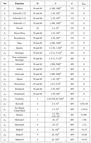
Table 2 presents the results of ABC-AX2 on the 30 standard benchmark functions and compares the results with the basic ABC [2] and ABC with self-adaptive mutation (ABC-SAM) [15]. All the algorithms have made 50 independent runs on each function and the mean and standard deviation of the best found solutions are presented in Table 2.

Fig. 2: Pseudocode for three-tier explorative tournament selection (on the left) and two-tier exploitative tournament selection (on the right) for ABC-AX2

Fig. 3: Search direction by ABC (on the left) and ABC-AX2 (on the right) in 2D search space

These algorithms have three parameters in common, which are population size SN, maximum cycle number MCN and

limit. For functions f1–f18 with D=30, ABC-AX2 used SN=100, MCN=1000 and limit=100. For the larger variants with D=60, the value of SN is kept the same (i.e., 100), but limit and MCN

are set to 200 and 2000, respectively. For the low dimensional

f19–f30, ABC-AX2 sets SN=100, MCN=100 and limit=10



D.

The other parameters of ABC-AX2 are set as: τ1=50, τ2=10,

u1=0.1, u2=0.5, qmin=1

D

,

qmax=1.0. Tournament sizes for

3T-ETS and 2T-ETS selection schemes (Fig. 2) are set as:

t1=t2=6, t3=4, and s1=6, s2=4. During initializations, control

parameter pi of each solution xi is set to 0.5, and the qi and ηij

values are initialized to random values from [qmin, qmax] and

[-1, 1], respectively. These values are chosen with some initial experiments and not meant for optimum. The results in Table 2 are summarized in the following points.

Algorithm: Two Tier Exploitative Tournament Selection(xi)

global P: Population of candidate solutions

global s1, s2: Tournament sizes for the similarity and

fitness based tournaments, respectively

return Tier2_Similarity_Tournament(xi)

procedure Tier2_Similarity_Tournament(xi)

best ← Tier1b_Fitness_Tournament() for i from 2 to s2 do

next ← Tier1b_Fitness_Tournament() if distance(next, xi) < distance(best, xi) then

best ← next

return best

procedure Tier1b_Fitness_Tournament()

best ← a solution picked at random from P for i from 2 to s1 do

next ← a solution picked at random from P if fitness(next) > fitness(best) then

best ← next

return best

Algorithm: ThreeTierExplorativeTournamentSelection(xi)

global P: Population of candidate solutions

global t1, t2,t3: Tournament sizes for the dissimilarity,

diversity and fitness based tournaments, respectively

return Tier3_Dissimilarity_Tournament(xi)

procedure Tier3_Dissimilarity_Tournament(xi)

best ← Tier2_Diversity_Tournament() for i from 2 to t3 do

next ← Tier2_Diversity_Tournament() if distance(next, xi) > distance(best, xi) then

best ← next

return best

procedure Tier2_Diversity_Tournament()

best ← Tier1a_Fitness_Tournament() for i from 2 to t2 do

next ← Tier1a_Fitness_Tournament() if diversity(next) > diversity(best) then

best ← next

return best

procedure Tier1a_Fitness_Tournament()

best ← a solution picked at random from P for i from 2 to t1 do

next ← a solution picked at random from P if fitness(next) > fitness(best) then

best ← next

 ABC vs. ABC-AX2: Out of the 18 high dimensional functions f1–f18, ABC-AX2 outperforms ABC on as many

as 16 functions, shows similar performance on one (f8),

while ABC manages to perform better only on one function (f7). Each time, the difference is statistically

significant, as measured by t-test with 99% confidence interval. For the low dimensional functions f19–f30, both

ABC and ABC-AX2 perform equally well on eight functions, while ABC-AX2 performs better on other four.

Table 1. Benchmark functions for experimental study. D: dimensionality of the function, S: search space, fmin: function value at global minimum, C: function characteristics with values — U: Unimodal,

M: Multimodal, S: Separable and N: Non-Separable.

No Function D S C fmin

f1 Sphere 30 and 60 [-100, 100]D US 0

f2 Schwefel 2.22 30 and 60 [-10, 10]

D

UN 0

f3 Schwefel 2.21 30 and 60 [-10, 10]D US 0

f4 Schwefel 1.2 30 and 60 [-100, 100]D UN 0

f5 Powell 24 [-4, 5]D UN 0

f6 Dixon-Price 30 and 60 [-10, 10]

D

UN 0

f7 Rosenbrock 30 and 60 [-30, 30]D UN 0

f8 Step 30 and 60 [-100, 100]D US 0

f9 Quartic 30 and 60 [-1.28, 1.28]

D

US 0

f10 Rastrigin 30 and 60 [-5.12, 5.12]D MS 0

f11

Non-continuous

Rastrigin 30 and 60 [-5.12, 5.12]

D

MS 0

f12 Schwefel 30 and 60 [-500, 500]D MS 0

f13 Ackley 30 and 60 [-32, 32]D MN 0

f14 Griewank 30 and 60 [-600, 600]

D

MN 0

f15 Alpine 30 and 60 [-10, 10]D MS 0

f16 Weierstrass 30 and 60 [-0.5, 0.5]D MS 0

f17 Penalized 30 and 60 [-50, 50]

D

MN 0

f18 Penalized2 30 and 60 [-50, 50]D MN 0

f19 Foxholes 2 [-65.536, 65.536]D MS 1

f20 Kowalik 4 [-5, 5]

D

MN 3.07e-04

f21

Six Hump

Camel Back 2 [-5, 5]

D

MN -1.0316

f22 Branin 2 [-5, 10]

x [0, 15] MS 0.398

f23 Hartman3 3 [0, 1]D MN -3.86

f24 Hartman6 6 [0, 1]

D

MN -3.32

f25 Shekel5 4 [0, 10]D MN -10.15

f26 Shekel7 4 [0, 10]D MN -10.40

f27 Shekel10 4 [0, 10]

D

f28 Fletcher Powell 10 [-π, π]D MN 0

f29 Michalewicz 10 [0, π]D MS -9.66015

f30 Langerman 10 [0, 10]D MN -1.4

Table 2. Comparison of ABC-AX2 with basic ABC [2] and ABC-SAM [15] on the standard benchmark suite functions. Best

results are marked with boldface font; if not other algorithms produce similar results.

No fmin D G ABC ABC-SAM ABC-AX

2

Mean Std. Dev. Mean Std. Dev. Mean Std. Dev.

f1 0

30 1000 2.45e–11 7.72e–12 4.18e–14 5.37e–15 5.51e–24 3.73e–25

60 2000 3.75e–10 2.01e–11 6.09e–13 7.24e–13 9.43e–28 7.26e–29

f2 0

30 1000 5.05e–07 1.74e–07 2.47e–08 2.35e–09 4.23e–15 3.54e–16

60 2000 5.58e–06 1.17e–06 5.06e–07 2.97e–07 2.98e–17 1.07e–17

f3 0

30 1000 4.18e+01 5.90 1.69e+01 1.43 6.60e–02 5.21e–03

60 2000 7.31e+01 6.88 3.10e+01 5.12 2.78 0.77

f4 0

30 1000 8.32e–10 9.75e–11 3.95e–12 5.77e–13 3.42e–16 8.83e–18

60 2000 4.50e–09 5.64e–10 7.54e–11 2.14e–11 8.84e–20 5.45e–21

f5 0 24 1000 6.61e+00 1.07e+00 9.24e–01 2.08e–01 2.23e–02 3.75e–03

f6 0

30 1000 6.67e–01 1.21e–08 2.16e–03 6.37e–04 5.91e–05 5.67e–06

60 2000 6.66e–01 1.05e–07 7.76e–02 1.63e–02 8.33e–05 1.71e–05

f7 0

30 1000 4.25e–01 1.18e–01 2.28e+01 3.75 2.39e+01 3.66

60 2000 2.02e–01 6.92e–02 4.96e+01 7.80 5.15e+01 7.69

f8 0

30 1000 0 0 0 0 0 0

60 2000 0 0 0 0 0 0

f9 0

30 1000 8.60e–13 8.32e–13 3.66e–16 1.44e–17 8.87e–34 6.78e–35

60 2000 9.31e–12 7.17e–12 4.76e–15 5.32e–16 6.31e–32 2.16e–33

f10 0

30 1000 1.72e–14 1.56e–14 1.26e–16 2.11e–17 4.68e–24 9.03e–26

60 2000 2.84e–13 8.01e–14 8.55e–15 3.15e–16 6.12e–31 8.67e–33

f11 0

30 1000 2.33e–08 7.49e–09 4.60e–10 8.85e–11 1.04e–13 3.16e–14

60 2000 6.64e–07 1.51e–07 6.80e–09 8.77e–10 4.25e–13 7.32e–14

f12

–12569.5 30 1000 –11346.79 2.77e+02 –12416.19 4.02e+01 –12569.48 1.50e–02

–25138.9 60 2000 –22530.82 4.08e+02 –23805.93 2.84e+02 –25016.6 1.89e+01

f13 0

30 1000 2.93e–06 3.38e–07 9.26e–08 1.89e–08 8.13e–13 6.71e–14

60 2000 4.65e–06 1.07e–06 2.07e–08 3.55e–08 3.62e–14 1.15e–15

f14 0

30 1000 4.55e–08 6.54e–09 8.36e–10 5.08e–11 5.63e–23 7.35e–25

60 2000 8.01e–07 2.64e–07 1.56e–10 6.90e–11 7.04e–31 5.77e–32

f15 0

30 1000 3.34e–04 3.76e–05 2.22e–08 3.93e–09 8.56e–13 1.56e–13

60 2000 7.49e–03 9.58e–04 1.17e–08 2.35e–09 5.37e–13 1.25e–13

f16 0

30 1000 3.36e–01 9.58e–02 5.78e–04 6.31e–05 6.46e–09 8.32e–10

60 2000 8.99e–01 3.09e–01 9.20e–03 4.03e–03 5.38e–08 9.19e–10

f17 0

30 1000 5.47e–12 2.09e–13 2.78e–12 8.89e–13 3.85e–14 4.93e–15

60 2000 7.47e–12 1.74e–12 1.32e–12 5.15e–13 3.50e–14 2.60e–15

f18 0

30 1000 2.63e–03 1.89e–04 3.06e–02 8.59e–03 2.33e–21 7.55e–22

60 2000 2.66e–03 7.90e–04 5.11e–02 7.39e–03 7.52e–26 1.29e–26

f19 1 2 100 1.04 0.04 1.03 0.03 1.01 0.01

f20 3.07e–04 4 100 5.98e–04 7.22e–05 4.32e–04 1.09e–05 3.10e–04 8.73e–06

f21 –1.0316 2 100 –1.0316 0 –1.0316 0 –1.0316 0

f22 0.398 2 100 0.398 7.12e–08 0.398 2.75e–07 0.398 1.83e–07

f23 –3.86 3 100 –3.86 7.09e–07 –3.86 1.54e–08 –3.86 6.77e–10

f24 –3.32 6 100 –3.32 4.74e–13 –3.32 6.26e–14 –3.32 2.61e–15

f25 –10.15 4 100 –9.61 0.14 –10.14 3.68e–07 –10.15 9.15e–08

f26 –10.40 4 100 –10.40 8.61e–03 –10.40 7.94e–03 –10.40 2.56e–03

f27 –10.54 4 100 –10.52 0.08 –10.54 6.77e–07 –10.55 7.84e–08

f28 0 10 100 13.77 3.80 4.02 0.39 4.19e–01 6.54e–02

f30 -1.4 10 100 –0.78 0.09 –1.04 0.06 –1.28 0.03

Summary (t-Test)

+ 20 19

– 1 0

≈ 9 11

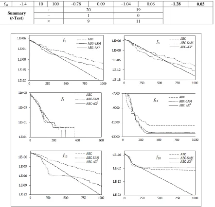
Fig. 4. Convergence characteristics of ABC, ABC-SAM and ABC-AX2 on three unimodal (f1, f4, f8)

and three multimodal (f12, f13, f18) functions. The vertical axis is the function value and the horizontal

axis is the number of cycles elapsed.

 ABC-SAM vs. ABC-AX2: On all of the 30 functions,

ABC-AX2 performs either better than or as well as ABC-SAM. For the high dimensional functions f1–f18,

ABC-AX2 significantly outperforms ABC-SAM on as many as 16 functions and shows similar performance on two (f7 and f8). On most (nine out of twelve) of the low

dimensional functions f19–f30, both perform equally well,

but ABC-AX2 performs better on the remaining three.

 For almost all the functions, ABC-AX2 shows very low standard deviation of its results. This indicates its high degree of consistency and robustness for all these benchmark functions.

 The ‗+‘, ‗–‘ and ‗≈‘ symbols at the bottom rows count the number of functions where ABC-AX2 _produces

significantly better, worse and similar results, respectively compared to ABC or ABC-SAM. Out of 30 functions, ABC-AX2 performs significantly better than ABC and ABC-SAM on 20 and 19 functions, shows

similar performance on 9 and 11 functions, while ABC performs better on one function (f7) only. So the overall

performance of ABC-AX2 is much better than others.

Fig. 4 shows the convergence graphs of ABC, ABC-SAM and ABC-AX2 for three unimodal (f1, f4, f8) and three multimodal

(f12, f13, f18) functions with D=30. ABC-AX2 shows far better

convergence characteristics than its counterparts for all these functions. For example, consider the functions f12 and f18,

where both ABC and ABC-SAM converges to a local minimum and gets stuck there till the end of their execution. In contrast, ABC-AX2 _{easily reaches the global minimum for} f12 and shows no sign of fitness stagnation for f18, even after

reaching the vicinity of the global minimum. For some functions, e.g., f1, f4, f13 and f18, ABC-SAM initially shows

somewhat higher convergence speed than ABC-AX2_{, but}

eventually it either gets stuck at local optima (f13, f18) or

gradually slows down (f1, f4) and at the end, ABC-AX2 shows

very close proximity to the global minimum, while ABC and ABC-SAM can get stuck at several intermediate local optima (note the semi-flat and flat regions of the plot of ABC in f4

and ABC-SAM in f13). Previously Table 2 considered the

performance of all three algorithms to be similar on f8, but

Fig. 4 now reveals that ABC-AX2 _{actually reaches the global}

minimum of f8 much earlier than both ABC-SAM and ABC.

Table 3. Comparison of ABC-AX2 _{with the CABC [16] variants. The boldface font marks the best performance for each}

function. The +, – and ≈ counts the number of instances where ABC-AX2 performs better, worse and similar, respectively.

Function CABC_S CABC_H ABC-AX

2

Mean Std. Dev. Mean Std. Dev. Mean Std. Dev.

f1 3.30e–19 2.00e-19 5.92e–18 3.56e–18 7.22e–51 4.08e–52

f7 6.33e+00 7.68e+00 4.80e–01 8.55e–01 5.94e+00 4.35e+00

f10 0 0 0 0 8.56e–54 3.83e–55

f12 1.30e–04 5.21e–06 1.27e–04 0 1.04e–06 7.98e–08

f13 1.83e–14 9.86e–15 8.35e–15 4.13e–15 7.14e–18 7.83e–19

f14 4.42e–02 2.99e–02 7.96e–03 9.06e–03 3.84e–54 2.04e–55

+ 4 4

– 1 2

≈ 1 0

Table 4. Comparison between ABC-AX2 and DABC [17]. Best results are marked with bold font; if not both the

algorithms produce identical results.

Function D DABC ABC-AX

2

Mean Std. Dev. Mean Std. Dev.

f1

10 2.01e–17 5.63e–17 0 0

30 2.01e–16 2.85e–17 7.26e–51 6.47e–52

f7

10 2.73e–03 7.04e–03 9.46e–02 8.22e–03

30 1.42e–02 2.53e–02 5.88e–01 8.32e–02

f10

10 0 0 0 0

30 0 0 0 0

f14

10 0 0 0 0

30 2.59e–16 1.22e–16 1.78e–50 5.28e–51

+ 2

– 1

≈ 1

Table 5. Comparison between ABC-AX2 and ChABC [18]. Best results are marked with bold font.

Function D CHABC ABC-AX

2

Mean Std. Dev. Mean Std. Dev.

f1 30 2.99e–16 3.54e–17 9.76e–119 7.17e–120

f7 30 6.33e–02 8.96e–02 8.48e–07 4.99e–08

f10 30 0 0 8.60e–129 5.14e–130

f12 30 3.81e–04 2.07e–04 5.32e–06 6.04e–07

f13 30 2.93e–14 2.99e–15 2.48e–17 4.09e–18

f14 30 2.70e–16 6.20e–17 1.85e–129 5.75e–130

– 1

≈ 0

Table 6. Comparison between ABC-AX2 and GABC [20]. Best results are marked with bold font.

Function D GABC (C=1.0) GABC (C=1.5) ABC-AX

2

Mean Std. Dev. Mean Std. Dev. Mean Std. Dev.

f1

30 4.31e–16 7.49e–17 4.17e–16 7.36e–17 9.66e–105 8.05e–106

60 1.43e–15 1.43e–16 1.43e–15 1.37e–16 1.98e–36 3.58e–37

f7

2 3.93e–04 4.45e–04 1.68e–04 1.45e–04 7.88e–03 5.35e–04

3 2.63e–03 2.11e–03 2.65e–03 2.22e–03 2.13e–01 6.12e–02

f10

30 9.47e–15 2.15e–14 1.32e–14 2.44e–14 6.30e–108 1.52e–109

60 4.16e–13 1.77e–13 3.52e–13 1.24e–13 7.42e–40 3.75e–41

f13

30 3.31e–14 2.90e–15 3.21e–14 3.25e–15 4.04e–19 8.28e–20

60 1.04e–13 1.07e–14 1.00e–13 6.08e–15 1.63e–17 2.66e–18

f14

30 8.88e–17 8.45e–17 2.96e–17 4.99e–17 9.50e–101 2.00e–102

60 9.47e–16 7.84e–16 7.54e–17 4.12e–16 1.81e–33 3.25e–34

+ 4 4

– 1 1

≈ 0 0

Table 7. Comparison of ABC-AX2 with HJABC [21] based onconvergence speed. Best results are marked with bold font.

Function D Number of function evaluations

HJABC ABC-AX2

f1 30 18322 13805

f2 30 12509 17987

f3 30 120315 –

f4 30 43939 35502

f7 30 102718 –

f8 30 17755 13986

f9 30 – 12230

f10 30 15376 20713

f13 30 54497 42609

f14 30 56855 31582

f15 30 99686 81678

+ 7

– 4

≈ 0

5.2

Comparison with other ABC-variants

In this section ABC-AX2 is compared with some other recent variants of ABC, such as the cooperative ABC (CABC) [16], ABC with diversity strategy [17], chaotic ABC (CHABC) [18], gbest-guided ABC (GABC) [20] and Hooke Jeeves ABC

(HJABC) [21]. The first three variants (e.g., [16]–[18]) increase the degree of explorations, while the last two variants (e.g., [20]–[21]) increase the intensity of exploitations.

First, ABC-AX2 _{is compared with CABC [16], which is a}

been introduced in two different versions — CABC_S and CABC_H. In order to perform more explorations, CABC_S decomposes the search space into multiple sub-spaces and employs different bee colonies to search and explore the different sub-spaces. The other variant, CABC_H tries to perform more exploitations than CABC_S by repeatedly alternating between explorative CABC_S and exploitative ABC. For comparison, ABC-AX2 is re-implemented with the same settings [16] — SN=40, no. of function evaluations

FE=100,000 and limit=SN



D. Table 3 shows that ABC-AX2 significantly outperforms both the CABC variants on four out of the six benchmark functions, while CABC_S and CABC_H perform better on one or two functions only. So the overall performance of ABC-AX2 is better than the CABC variants.

The next comparison is made between ABC-AX2 and DABC [17]. DABC tries to maintain sufficient amount of diversity among the candidate solutions to allow more search space explorations. DABC regularly measures the existing population diversity d and employs either its explorative or exploitative perturbation based on the value of d. ABC-AX2 is re-implemented with SN=20, MCN=5000 and limit=100 to compare with DABC. Results presented in Table 4 show that ABC-AX2 performs better than DABC on two out of four functions (f1 and f14), shows similar performance on one (f10),

while DABC performs better on the remaining one function (f7) only. The reason may be that DABC completely relies on

its estimated value of population diversity d to choose between explorations and exploitations, while there is no accurate metric for diversity. Besides, DABC uses a naïve strategy of fixed threshold diversity value (dlow in [17]), which

may cause repeated oscillations between conflicting explorations and exploitations to reduce convergence speed.

Next, ABC-AX2 is compared with the Chaotic ABC (CHABC) [18] algorithm. CHABC employs chaotic search behavior during perturbations to produce new food positions from the existing ones. Chaotic dynamics are produced by the logistic equations (eq. (4)–(7) in [18]) which provide a simple mechanism to escape from local minima and avoid premature convergence. For comparison, ABC-AX2 is executed for 5000 cycles with population size of 70 and limit=200, as suggested in [18]. Results (Table 5) show that ABC-AX2 outperforms CHABC on as many as five out of the six functions, while CHABC performs better on the remaining one function (f10)

only. The reason may be that CHABC employs same chaotic strategy uniformly for all the candidate solutions across the population, without considering their individual exploitative/explorative requirement, while ABC-AX2

considers and customizes the degree of explorations and exploitations separately for every candidate solution.

Next, ABC-AX2 is compared with GABC [20], which is an exploitative ABC-variant that tries to improve the convergence speed by using the information of the global best solution found so far into the perturbation scheme (1). ABC-AX2 is executed with the same settings [20] and results are presented in Table 6. In [20], GABC is tested with several values of its parameter C, but the best results are always observed with C = 1.0 or 1.5, so Table 6 includes both the results. Results show that ABC-AX2 outperforms GABC on four out of the five functions, while GABC performs better on the remaining one (f7) only. The reason may be that the

perturbation operation of GABC becomes too exploitative by pushing its candidate solutions towards the best solution found so far. Increased exploitations, at the cost of reduced

explorations, may improve the final solution quality for the unimodal and low dimensional function f7, but is likely to fail

for the other four multimodal functions in Table 6.

Next, ABC-AX2 is compared with HJABC [21], which is a hybrid ABC-variant that intensifies the degree of exploitations by hybridizing basic ABC with an efficient local search technique (i.e., Hooke Jeeves pattern search). Table 7 compares ABC-AX2 and HJABC based on the number of function evaluations (NFE) required to achieve a predefined level of accuracy. Both ABC-AX2 and HJABC are run with

SN=25 and limit=SN



D, until either NFE reaches a predefined maximum value (NFEmax) or the algorithm reaches

as accuracy of ɛ around the global minimum. As suggested in [21], ABC-AX2 used ɛ = 10-8 with NFEmax=300000. For seven

out of the eleven functions in Table 7, ABC-AX2 performs better than HJABC, by showing a faster convergence speed, while HJABC performs better on the remaining four. However, ABC-AX2 can‘t achieve the predefined level of accuracy within NFEmax function evaluations for two

functions (f3 and f7), while HJABC fails to do so only for one

function (f9). In short, the overall performance of ABC-AX2 is

quite comparable to HJABC. The reason that HJABC often requires larger number of function evaluations, even after using the efficient Hooke Jeeves local searcher [21], may be that HJABC regularly tries to find an appropriate search direction by exploring along the axis directions only, exploring just one variable at a time, which is not suitable for the non-separable problems.

6.

CONCLUSION AND SUGGESTION

FOR FURTHER STUDY

This paper introduces ABC-AX2 — an improvement of the basic ABC algorithm [2] that tries to adaptively control the degree of explorations and exploitations, separately for each candidate solution. ABC-AX2 includes three control parameters — pi, qi and ηiwithin each candidate solution xi

and employs adaptive and self-adaptive techniques to adapt their values gradually. The control parameter pi controls the

proportion of exploitative and explorative perturbations on xi

and is gradually adapted by ABC-AX2 based on the previous successes and failures of the exploitative and explorative perturbations on xi. The other two control parameters – qi and ηicontrol the perturbation rate and perturbation scaling factors

for xi and they have to go through gradual self-adaptation, using (8) and (10) respectively.

ABC-AX2 significantly differs from most other existing variants of ABC algorithm. Most ABC-variants view exploitations and explorations as conflicting operations, so they try to improve either the local exploitations (e.g., GABC [20], HJABC [21]) or the global explorations (e.g., CABC [16], DABC [17], CHABC [18]) of the basic ABC algorithm, without trying to establish a proper balance between exploitations and explorations. In contrast, ABC-AX2 considers exploitations and explorations to be complementary, rather than conflicting, operations and try to achieve some degree of both exploitations and explorations throughout the entire optimization procedure. For example, ABC-AX2 keeps the value of pi always within [0.1, 0.9] to avoid the complete

domination by either exploitative or explorative perturbations. Also, ABC-AX2 _{uses fixed values of u}

1 and u2 (e.g., 0.1 and

0.5, respectively, as in the current implementation), so there is always significant possibility that the values of qi and ηiwill

induce both explorations and exploitations on xi throughout the entire optimization procedure. Experimental results (Tables 2–7) clearly show that ABC-AX2 has significantly improved its results over the basic ABC algorithm [2] as well as several other recent variants of ABC (e.g., [15]–[21]).

There may be several possible future research directions based on this study. Firstly, ABC-AX2 uses a simple strategy to adjust the control parameters – pi, qi and ηifor each candidate

solution xi. A more sophisticated strategy, such as considering

the properties of fitness landscape around xi, or using a strategy parameterized by existing population diversity or the maturity of the optimization process may be more effective to balance between exploitations and explorations around xi.

Secondly, the quality of the final solution could be improved further by using an exploitative and efficient local searcher. This may pinpoint the global minimum more precisely. Thirdly, ABC-AX2 _{can be hybridized with many other}

existing evolutionary, swarm intelligence, machine learning techniques to further improve its results. Finally, ABC-AX2 has been employed on the continuous problems. It would be interesting to know how well ABC-AX2 performs on other existing problems, especially the discrete and real world ones.

7.

REFERENCES

[1] D. Karaboga, ―An idea based on honey bee swarm for numerical optimization‖, Erciyes University, Kayseri, Turkey, Technical Report-TR06, 2005.

[2] D. Karaboga, B. Akay, ―A comparative study of artificial bee colony algorithm‖, Applied Mathematics and Computation 214 (1) (2009) 108–132.

[3] Q. Bai, X. Yun, ―A new hybrid artificial bee colony algorithm for the traveling salesman problem‖, in: Proc. 3rd Int. Conf. Communication Software and Networks (ICCSN), 2011, pp. 155–159.

[4] N. Stanarevic, M. Tuba, N. Bacanin, ―Modified artificial bee colony algorithm for constrained problems optimization‖, Int. Journal of Mathematical Models and Methods in Applied Sciences 5 (3) (2011) 644–651. [5] S. Omkar, J. Senthilnath, R. Khandelwal, G. Naik, S.

Gopalakrishnan, ―Artificial bee colony (ABC) for multi-objective design optimization of composite structures‖, Applied Soft Computing 11 (1) (2011) 489–499. [6] F. Kang, J. Li, Q. Xu, ―Structural inverse analysis by

hybrid simplex artificial bee colony algorithms‖, Computers and Structures 87 (13–14) (2009) 861–870. [7] R. Irani, R. Nasimi, ―Application of artificial bee

colony-based neural network in bottom hole pressure prediction in underbalanced drilling‖, Journal of Petroleum Science and Engineering 78 (1) (2011) 6–12.

[8] N. Karaboga, ―A new design method based on artificial bee colony algorithm for digital IIR filters‖, Journal of the Franklin Institute 346 (4) (2009) 328–348.

[9] D. Karaboga, B. Akay, ―PID controller design by using artificial bee colony, harmony search and bees algorithms‖, in: Proceedings of the Institution of Mechanical Engineers, Part I: Journal of Systems and Control Engineering 224 (7) (2010) 869–883.

[10]R. Rao, P. Pawar, ―Parameter optimization of a multi-pass milling process using non-traditional optimization algorithms‖, Applied Soft Computing 10 (2) (2010) 445-456.

[11]D. Karaboga, B. Gorkemli, C. Ozturk, N. Karaboga, ―A comprehensive survey: artificial bee colony (ABC) algorithm and applications‖, Artificial Intelligence Review (2012) 1–37.

[12]L. Bao, J. Zeng, ―Comparison and analysis of the selection mechanism in the artificial bee colony algorithm‖, in: Proc. 9th Int. Conf. Hybrid Intelligent Systems, 2009, pp. 411–416.

[13]W. Gao, S. Liu, ―A modified artificial bee colony algorithm‖, Computers and Operations Research 39 (3) (2012) 687–697.

[14]J. Lampinen, I. Zelinka, ―On stagnation of the differential evolution algorithm‖, in: Proc. 6th Int. Mendel Conf. on Soft Computing, 2000, pp. 76–83. [15]M. S. Alam, M. M. Islam, ―Artificial bee colony

algorithm with self-adaptive mutation: A novel approach for numeric optimization‖, in: Proc. 2011 IEEE Int. Conf. on Trends and Developments in Converging Technology (TENCON), 2011, pp. 49–53.

[16]M. Abd, ―A cooperative approach to the artificial bee colony algorithm‖, in: IEEE Congress on Evolutionary Computation (CEC), 2010, pp. 1–5.

[17]W. Lee, W. Cai, ―A novel artificial bee colony algorithm with diversity strategy‖, in: Proc. 7th Int. Conf. Natural Computation, 2011, pp. 1441–1444.

[18]B. Wu, S. Fan, ―Improved Artificial Bee Colony Algorithm with Chaos‖, in: Y. Yu, Z. Yu, J. Zhao (Eds.): Computer Science for Environmental Engineering and EcoInformatics, Part I, Communications in Computer and Information Science, vol. 158, 2011, pp. 51-56. [19]L. Fenglei, D. Haijun, F. Xing, ―The parameter

improvement of bee colony algorithm in TSP problem‖, Science Paper Online, November 2007.

[20]G. Zhu, S. Kwong, ―Gbest-guided artificial bee colony algorithm for numerical function optimization‖, Applied Mathematics & Computation 217 (7) (2010) 3166–3173. [21]F. Kang, J. Li, Z. Ma, H. Li, ―Artificial bee colony

algorithm with local search for numerical optimization‖, Journal of Software 6 (3) (2011) 490–497.

[22]F. Qingxian, D. Haijun, ―Bee colony algorithm for the function optimization‖, Science Paper Online, 2008. [23]H. Quan, X. Shi, ―On the analysis of performance of the

improved ABC algorithm‖, in: 4th IEEE Int. Conf. Natural Computation (ICNC), 2008, pp. 654–658. [24]E. Montes, R. Koeppel, ―Elitist artificial bee colony for

constrained real-parameter optimization‖, IEEE Congress on Evolutionary Computation 11 (2010) 1–8. [25]S. Nieberg, H. Beyer, ―Self-adaptation in evolutionary

algorithms‖, Parameter Setting in Evolutionary Algorithm (2007) 47–76.

[26]J. Liang, A. Qin, P. Suganthan, S. Baskar, ―Comprehensive learning particle swarm optimizer for global optimization of multimodal functions‖, IEEE Trans. on Evolutionary Comput. 10 (3) (2006) 281--295. [27]C. Lee, X. Yao, ―Evolutionary programming using

mutations based on the Lévy probability distribution‖, IEEE Transactions on Evolutionary Computation 8 (1) (2004) 1–13.