www.nat-hazards-earth-syst-sci.net/13/2369/2013/ doi:10.5194/nhess-13-2369-2013
© Author(s) 2013. CC Attribution 3.0 License.
Natural Hazards
and Earth System
Sciences
Estimating soil suction from electrical resistivity
E. Piegari and R. Di Maio
Department of Earth Sciences, Environment and Resources, University of Naples “Federico II”, Largo San Marcellino 10, 80138 Naples, Italy
Correspondence to: E. Piegari ([email protected])
Received: 27 October 2011 – Published in Nat. Hazards Earth Syst. Sci. Discuss.: – Revised: 3 April 2013 – Accepted: 23 June 2013 – Published: 26 September 2013
Abstract. Soil suction and resistivity strongly depend on the
degree of soil saturation and, therefore, both are used for es-timating water content variations. The main difference be-tween them is that soil suction is measured using tensiome-ters, which give point information, while resistivity is ob-tained by tomography surveys, which provide distributions of resistivity values in large volumes, although with less ac-curacy. In this paper, we have related soil suction to electri-cal resistivity with the aim of obtaining information about soil suction changes in large volumes, and not only for small areas around soil suction probes. We derived analytical re-lationships between soil matric suction and electrical resis-tivity by combining the empirical laws of van Genuchten and Archie. The obtained relationships were used to evalu-ate maps of soil suction values in different ashy layers orig-inating in the explosive activity of the Mt Somma-Vesuvius volcano (southern Italy). Our findings provided a further ex-ample of the high potential of geophysical methods in con-tributing to more effective monitoring of soil stress condi-tions; this is of primary importance in areas where rainfall-induced landslides occur periodically.
1 Introduction
Soil suction plays a crucial role in affecting slope equilib-rium conditions. In particular, if the thickness of the un-saturated zone is large and the slope inclination is greater than the soil’s internal friction angle, stability is mainly trolled by the apparent cohesion due to suction, which con-tributes to the shear strength of unsaturated soils. During in-tense rainfall, water infiltration processes cause a decrease in suction, which may induce slope failure. Such conditions are realized in the Campanian pyroclastic soils (southern
Italy), which cover the relatively steep slopes around the Mt Somma-Vesuvius volcano and have constituted a serious and recurring hazard for densely urbanized areas in the vicin-ity since historical times (de Riso and Nota d’Elogio, 1973; Guadagno, 1991).
Several authors suggest that field monitoring of soil suc-tion is an essential tool in effective early warning systems (Cascini and Sorbino, 2002; Olivares and Tommasi, 2008; Pagano et al., 2008; Greco et al., 2010; Toll et al., 2011). A large number of soil suction measurements have been collected over an area of about 3000 km2 and, at the same time, accurate laboratory investigations have been performed on unsaturated samples from the Pizzo D’Alvano massif, Cervinara and other localities of the Salerno and Avellino provinces (Cascini and Sorbino, 2002). In particular, it has been found that suction values are quite low in the pyroclas-tic soils affected by the flow slides that occurred in May 1998 on the Sarno mountains (Evangelista et al., 2001); the max-imum values – at each site and at any investigated depth – did not exceed 65 kPa and minimum values of about 1–2 kPa were recorded in the period from January to May (Cascini and Sorbino, 2002). Interestingly, during the period covering the end of the winter and the beginning of the spring, pyro-clastic cover seems to attain high values of saturation at all depths, with mean suction values ranging, at any location, from 5 to 10 kPa (Cascini and Sorbino, 2002). However, soil suction measurements, even when made over large areas, can only provide time variations of water content at a given point and, therefore, the spatial variability of soil water content in the field cannot be clearly understood.
they are non-invasive techniques, enabling the variations of some physical quantities in large buried volumes to be mea-sured; this is in contrast to remote sensing or aerial photogra-phy, which can only provide surface information, or to bore-hole and penetration tests, which only provide subsurface data in small volumes around porous probes. In particular, the well-known dependence of electrical resistivity values on the geostructural properties and water content of soils sug-gests the geoelectrical method as one of the most suitable for studying landslide risk.
Repeated time-lapse resistivity surveys have been carried out to analyse the effects of saturation in areas susceptible to landsliding (Suzuki and Higashi, 2001; Friedel et al., 2006; Jomard et al., 2007; Di Maio and Piegari, 2011), and a con-ceptual model has been proposed to relate time-lapse resis-tivity changes to slope failure of pyroclastic covers (Piegari et al., 2009; Di Maio and Piegari, 2012). Moreover, auto-mated resistivity tomography systems with permanently in-stalled electrode networks have now been implemented to monitor soil conditions surrounding a number of active land-slides (Supper et al., 2008; Chambers et al., 2009; Lebourg et al., 2009).
Since both suction and electrical resistivity are physical quantities that strongly depend on water content in the field, it is reasonable to ask if they are correlated. Recently, De Vita et al. (2012) have performed geophysical and geotechnical laboratory analyses on pairs of pyroclastic samples collected from the same sites in an area susceptible to debris-flow land-slides, and have studied the correlation between electrical re-sistivity and matric suction in these soils. On the basis of such a study, in this paper we propose a non-invasive method for monitoring spatial variations of soil suction by using soil resistivity data derived from in situ electrical resistivity to-mography surveys. An application of the proposed approach in a test area is presented.
2 A relationship between resistivity and soil suction
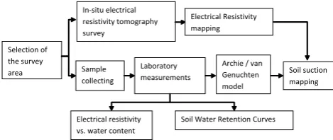
A schematic diagram (Fig. 1) shows our proposal for carry-ing out soil suction mappcarry-ing. Startcarry-ing from in situ resistivity data obtained by electrical resistivity tomography (ERT) sur-veys in an area susceptible to debris-flow phenomena, we cal-ibrated these measurements through laboratory experiments performed on samples collected from different depths of the selected cover. From the fit of the data, we obtained values for the empirical parameters of Archie’s law (Archie, 1942). These parameters were used to invert the Archie relationship and to introduce the dependence on resistivity into the van Genuchten expression (van Genuchten, 1980), which relates water retention data to soil suction. In this way, we obtained a closed-form model that is a combination of the Archie and van Genuchten empirical laws and can be applied to predict-ing matric suction values by uspredict-ing resistivity data. A possi-ble application of the proposed algebraic expression consists
16 Selection of
the survey area
In-situ electrical resistivity tomography survey
Sample collecting
Laboratory measurements
Electrical resistivity vs. water content
Soil Water Retention Curves
Soil suction mapping Electrical Resistivity
mapping
Archie / van Genuchten model
1
Fig. 1.Schematic diagram of the proposed procedure for carrying out soil suction mapping. 2
3
Eliminato: ure 4
Fig. 1. Schematic diagram of the proposed procedure for carrying
out soil suction mapping.
in determining soil suction maps at different depths across large areas, unlike tensiometer measurements, which provide punctual suction values.
In the following description, we provide details of the pro-posed procedure and outline the assumptions on which it is founded.
ERT is one of the most widely used non-invasive tech-niques for studying geological and engineering problems (e.g. Jongmans and Garambois, 2007). The resistivity tomo-graphic approach, in fact, provides a very detailed image of subsurface resistivity distribution on the basis of rock and soil resistivity contrasts. For this reason, it is particularly well suited for characterizing the Campanian geological setting, which is susceptible to landslides, due to the high resistivity contrasts between the pyroclastic soils and the carbonate (or lava) rock basement. These contrasts are mainly governed by the different capacity of soils and rocks to retain water. Therefore, in order to quantify correctly variations in elec-trical resistivity in terms of water content, knowledge of the empirical relationships between these two physical quantities is required for the soils under examination.
The most common empirical quantitative relationship be-tween porosity, electrical resistivity and saturation of rocks is Archie’s law (Archie, 1942):
ρ=ρwϕ−mS−n, (1)
whereρ andρw are, respectively, the bulk resistivity of the
rock and the resistivity of the water,ϕis the porosity,mis the cementation exponent, which is related to the permeability of the rock and has values near to 1.3 for unconsolidated sands and ranging from 1.6 to 2 for consolidated sandstones.Sis the water saturation andnis the saturation exponent (related to the wettability of the rock), with values usually close to 2. Equation (1) is not the only form in which Archie’s law is written. There are several versions of Archie’s law, which attempt to include the effects of partial saturation or the pres-ence of mixed fluids or air in the vadose zone (Glover et al., 2000 and references therein). Furthermore, it is not valid for rocks composed of conducting matrix minerals and which have a significant percentage of clay contributing to the ma-trix conduction. For these reasons, even if our samples were clay free, we did not simply apply Eq. (1) to our laboratory
resistivity data, but fit them with different functions of the measured water content,θw. In this way, we could determine
the most accurate relationshipρ=ρ (θw)for the soils under
examination.
The most commonly monitored variable for predicting soil water storage is matric suction, the dependence of which on water content is described by the water retention curve, which is variable among different types of soil. Several mod-els have been proposed to characterize the shape of the water retention curve, and one of the most widely adopted is the van Genuchten model (1980):
θw=θr+
θs−θr
1+ |αh|n
n−1
n
, (2)
wherehis the suction pressure (cm of water),θs is the
sat-urated water content, θr is the residual water content,α is
related to the inverse of the air entry suction,α >0 (cm−1), andnis a measure of the pore-size distribution,n >1 (di-mensionless).
Taking into account the numerical factors that correlateh to matric suctions(kPa), Eq. (2) can be written as
s=1 ¯
α "
θw−θr
θs−θr
1−nn
−1 #n1
. (3)
If the volumetric water content in Eq. (3),θw, is expressed
in terms of the electrical resistivity by means of fitting func-tions to resistivity data, we obtain closed-form expressions for the matric suctions=s (ρ). In other words, we make ex-plicit the dependence ofson resistivity and, in the following, we describe how we used this to evaluate soil suction maps starting from electrical resistivity tomography data.
In the next section, we show an application of the proposed procedure in a test area of the Campania Region susceptible to debris-flow phenomena.
3 Soil suction maps of the Pizzo d’Alvano study area
(Campania Region, Italy)
3.1 Geological setting
The pyroclastic soils that cover many Campanian slopes originate from the eruptive activities of the Campi Flegrei, Ischia and Vesuvius volcanic districts. Such soils are also found at many tens of kilometres from the primary vol-canic vents, owing to aeolian transport of the eruption prod-ucts. Due to their typical vesicular structure, soils derived from ash-fall pyroclastic deposits have special engineering– geological properties, such as low values of dry unit weight and very high values of void ratio and porosity (Esposito and Guadagno, 1998; Bell, 2000). In particular, pyroclasts pre-vail in ash-fall pyroclastic deposits of Mt Somma-Vesuvius. Fine ash detritus (∅<1/16 mm) is constituted mainly of
bubble-wall shards derived from broken bubbles or vesicle walls (Fisher and Schmincke, 1984). Conversely, in coarse ash (1/16<∅<2 mm) and lapilli (∅>2 mm), pumiceous fragments can form pyroclasts that have completely or par-tially isolated intra-particle voids, therefore having a unit weight lower than the unit weight of water (9.807 kN m−3) and thus forming materials that are able to float (Fisher, 1961; Schmidt, 1981). However, sinking tests conducted on such volcanic materials reveal that pumiceous pyroclasts sink in water after a prolonged time due to the interconnections be-tween the intra-particle voids (Whitam and Sparks, 1986; Es-posito and Guadagno, 1998). This result suggests a different significance should be attributed to both inter-particle and intra-particle pore types, the contributions of which to the total porosity are critical for characterizing the peculiar wa-ter retention capacity of pumiceous pyroclasts. In particular, the presence of two different types of pores may explain the change in the decreasing rate of electrical resistivity for lower water contents (see Sect. 3.2.2).
Following the calamitous event of May 1998, the pyroclas-tic covers of Mt Pizzo D’Alvano (located at about 17 km east of Mt Somma-Vesuvius volcano) have been the subject of a large number of experimental investigations (Cascini et al., 2000; Chirico et al., 2000; Calcaterra et al., 2004; Crosta and Dal Negro, 2003; De Vita et al., 2006).
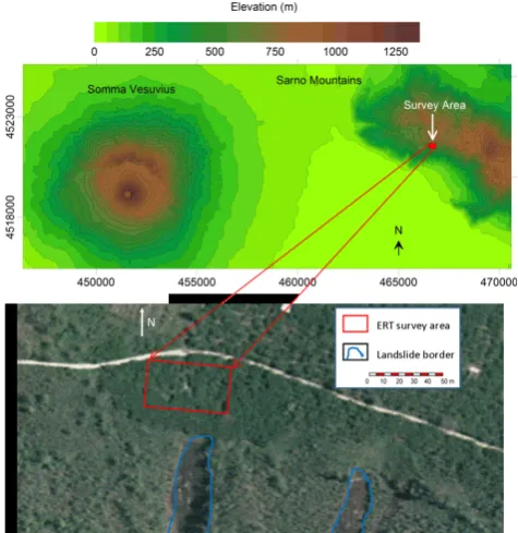
Our study area is located above the initial detachment ar-eas of two landslides that occurred on 5 and 6 May 1998 at Mt Pizzo d’Alvano (Fig. 2). The thickness of the pyro-clastic cover ranges mainly from 2 to 5 m depth and lies on a highly fractured carbonate bedrock with open joints filled by pyroclastic soil. The typical stratigraphic column of pyroclastic soil for the sample area, classified using litho-logical and pedolitho-logical criteria (Terribile et al., 2000) and the Unified Soil Classification System (Holtz and Kovacs, 1981), is as follows: A – humus (peat); B – very loose py-roclastic horizons subjected to highly pedogenetic processes with dense root apparatuses (silty sand); C – a very loose pumiceous lapilli horizon with a low degree of weather-ing (well-graded gravel, fine to coarse gravel–poorly graded gravel); Bb – buried soil or palaeosoil (silty sand); Cb – very loose pumiceous lapilli with a low degree of weather-ing (well-graded gravel, fine to coarse gravel–poorly graded gravel), corresponding to a deposit from the preceding erup-tion; Bbbasal) – basal buried palaeosoil (silty sand),
corre-sponding to intensely pedogenized pyroclastic deposits; R – fractured carbonate bedrock with open joints filled by soil derived from the above palaeosoil horizon.
3.2 Processing of resistivity data
3.2.1 Analysis of electrical resistivity tomography data
Fig. 2. Geoelectrical survey area (red rectangle) on an
orthophoto-graph of the northern slope of Mt Pizzo d’Alvano (Salerno, Italy). Blue lines indicate the initial detachment areas of two landslides that occurred on 5 and 6 May 1998.
Piegari, 2011, 2012). The data were collected using an IRIS-SYSCAL PRO System, with a multielectrode cable with electrodes spaced at 2 m intervals along the cable. A Wenner–Schlumberger array was used with a minimum and maximum current electrode separation of 6 and 44 m, respec-tively, and a minimum potential electrode separation of 2 m, giving a total number of measurements of 167 for each line and an investigation depth of about 10 m below ground level (b.g.l.). Since it is well known that the geophysical data in-version is affected by the problems of non-uniqueness of the solution and a decrease of the resolution with depth, we as-sessed the robustness of our model by analysing the depen-dence of the inversion results on the reference model, and by estimating the depth of interest (Oldenburg and Li, 1999; Hillbich et al., 2009).
The depth of interest (DOI) is a dimensionless parame-ter that measures how well the data are able to constrain the model. It was first introduced by Oldenburg and Li (1999) and is defined by
DOI(x, z)=m1(x, z)−m2(x, z)
m01−m02
,
wherem1andm2are the models provided by the inversion
of the resistivity data set through using two constant refer-ence models,m01 andm02, respectively. If the DOI value is
close to 0, the two inversions produce the same result and the model is well constrained by the data. If the DOI value is
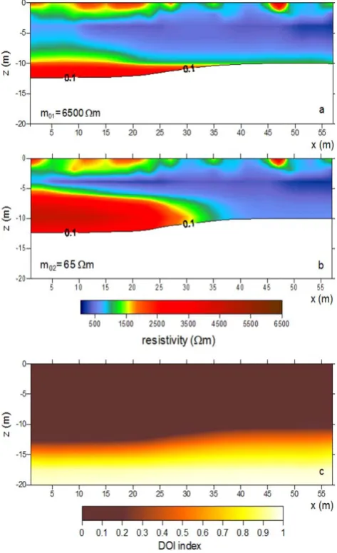
close to 1, the inversion is controlled by the reference models and the influence of the data is negligible. As an example, Fig. 3c shows the DOI index computed for one of the nine 2-D ERT profiles performed in the survey area. The average of the observed apparent resistivity data set was 650m. The two reference models were one-tenth and ten times such a value, i.e.m01=65m and m02=6500m. The two
in-versions were carried out using both the standard and the robust Gauss–Newton algorithm with the 2D inversion pro-gram RES2DINV (Loke and Barker, 1996; Loke, 2002; Loke and Dahlin, 2002). Figure 3a and b show the result for the two inversions obtained by the robust Gauss–Newton algo-rithm, with a cut-off value that was set according to a DOI index>0.1 (Oldenburg and Li, 1999; Hillbich et al., 2009). The resulting resistivity images were very similar, confirm-ing that the whole thickness of the pyroclastic cover is rea-sonably well resolved. Figure 4a shows the apparent resis-tivity values observed for the considered ERT profile, while Fig. 4c and b display, respectively, the model recovered from the inversion with a reference model of 650m and the pre-dicted resistivity data. Figure 4c also shows an overlaying of the DOI values from Fig. 3c.
Since we were interested in characterizing the whole pyro-clastic cover in terms of electrical resistivity values, we used the results derived from the DOI analysis of the 2-D ERT pro-files, in order to interpret the model that was generated using a pseudo 3-D resistivity inversion of the collected 2D appar-ent resistivity data (Di Maio and Piegari, 2011, 2012). The data were inverted by using the RES3-DINV program (Loke and Barker, 1996; Loke, 2002; Loke and Dahlin, 2002). In particular, we employed the finite element method to link the model parameters to the 3-D model response, and the complete Gauss–Newton technique to determine the change in the model parameters. The surface topography was sur-veyed and incorporated into the resistivity model. In Fig. 5, a clipped volume obtained by the 3-D inversion of the 2-D ERT data collected in the autumn is shown. In particular, the clip plane corresponds to the resistivity section shown in Fig. 4c. From the 3-D image, a decreasing trend of resistiv-ity with depth along about 4–5 m b.g.l. is evident; resistivresistiv-ity then starts to increase going downwards. We attributed this increase in resistivity with depth to the interface between the pyroclastic soils and the underlying highly fractured carbon-ate bedrock.
3.2.2 Analysis of laboratory resistivity data
Concurrently with the geoelectrical surveys, two sets of fif-teen undisturbed samples (cylinders with inner diameter: 74 mm; length: 148 mm), belonging to the B, Bb and Bbbasal
horizons, were collected from sampling pits located between about 10–20 m upstream of the main scarps: one set was used in the laboratory for engineering–geological analyses and the other for geophysical measurements. Details of the soil sample collecting methods are described in De Vita et
Fig. 3. Inverted resistivity models with factors (a) 0.1 and (b) 10 of
average apparent resistivity with a cut-off according to a DOI index
>0.1. (c) The calculated depth of interest index.
al. (2012). The fifteen samples used in geophysical analyses were saturated with rainwater (electrical conductivity σ=
88 µS cm−1) at room temperature and standard pressure to reproduce the in situ conditions.
Electrical measurements were performed starting from the saturated condition and then at decreasing levels of saturation (produced by drying the samples in an oven at a tempera-ture of 70◦C) up to completely dry conditions. The electrical measurements were carried out using the four-electrode tech-nique in the Wenner electrode array configuration (Vinegar and Waxman, 1984), to minimize the electrode polarization phenomena that can occur when a two-electrode array is ap-plied (Roberts and Lin, 1997; Taylor and Barker, 2002). Both the measurements of electrical resistivity and total sample weight were performed about 6 h after kiln-drying, in order to allow the samples to reach thermal equilibrium with the
environment at room temperature. At the end of the drying process, the corresponding gravimetric water content,w, was obtained from the ratio of the water and the oven-dried sam-ple weights (ASTM D 2216-80) for each measurement of re-sistivity and total sample weight. The volumetric water con-tent,θw, was obtained as the product of the gravimetric water
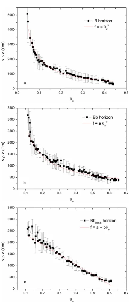
content and the soil’s dry unit weight divided by the water unit weight. A detailed description of the experimental set-ting and procedure is given in De Vita et al. (2012). Here, we summarize the results of the laboratory study by plotting for each horizon the sample-averaged resistivity as a function of the volumetric water contentθw(Fig. 6). Since we are
inter-ested in characterizing the average response of the ashy lay-ers to the electric current flow, we considered the average of the laboratory resistivity values corresponding to similar wa-ter contents for the three investigated soil types. However, the relationship between resistivity and volumetric water content showed some scatter within each of the three soil types, as is shown in De Vita et al. (2012). The scatter of the data reflects the heterogeneity of natural soils and, therefore, we took into account the observed spread of data values by range, i.e. the difference between the highest and the lowest observed resis-tivity values. In Fig. 6a, b and c, we show average values of ρand range bars for each data set. The average values were calculated for six samples belonging to the B and Bb hori-zons, and for three samples of the Bbbasalhorizon. We noted
that, due to the natural heterogeneity of samples, the number ofρ values measured in a given water content interval was variable (ranging from 1 to 6 for samples from the B and Bb horizons, and from 1 to 3 for samples from the Bbbasal
hori-zon). When only a single sample resistivity value was found in a given water content interval, this value was considered the least accurate datum. Indeed, in this case, it was not pos-sible to calculate the data spread and, according to the most cautious choice, we attributed to this single value the largest observed error bar. It is also worth noting that resistivity data from laboratory measurements were also affected by errors associated with the experimental procedure. We verified that the measurement errors were much smaller than the intrinsic dispersion related to the heterogeneity of the samples, and the related error bars were smaller than or equal to the sym-bol sizes employed.
In order to obtain analytical functions relating resistivity to water content, we fit the data shown in Fig. 6a, b and c. The values of the best fitting parameters are reported in Ta-ble 1. They were derived from weighted non-linear and linear least squares regressions, in which the weights were taken as equal to 1/σi2, withσibeing the range bar sizes shown in the
plots in Fig. 6. The goodness of fit tests were evaluated by the values of the reduced chi square,χ¯2, and the coefficient of determination, R¯2. To improve the curve-fitting results, we considered only water content values larger than 10 % for the deepest layers (i.e. the Bb and Bbbasal horizons). Such a
Fig. 4. Apparent resistivity data from the considered 2-D ERT profile are shown in (a), while the calculated apparent resistivity data are in (b). The model recovered from the inversion, with a reference model equal to the average of the collected apparent resistivity data (650m), is in (c). The DOI values of Fig. 3c are superimposed on the model with a contour line interval of 0.1.
20 1
2
Fig. 5. Resistivities of the investigated buried volume obtained from the results derived from
3
the 3D data inversion for the autumn survey. 4
5
Eliminato: ure
6
Eliminato: of
7
Eliminato: al
8
Fig. 5. Resistivities of the investigated buried volume obtained from
the results derived from the 3-D data inversion for the autumn sur-vey.
content induced by rainfall. The numerical analysis deter-mined that the resistivity curves of the B and Bb horizons were well described by power laws (Fig. 6a, b), such as the Archie relationship. Instead, the behaviour ofρ in relation to the lowest pyroclastic horizon (Fig. 6c), which, unlike the other horizons, is composed of a small percentage of clay (De Vita et al., 2012), appeared to be better described by a linear dependence on the water content.
3.3 Relationships between soil suction and resistivity for
the examined soil horizons
The soil water retention curves for the pyroclastic samples collected in the survey area (see Sect. 3.2), which are repre-sentative of the B, Bb and Bbbasalhorizons (see Sect. 3), have
been reconstructed by De Vita et al. (2012). In Table 2, we re-port the estimated value of the van Genuchten model param-eters obtained by means of RETC software (van Genuchten, 1980; van Genuchten et al., 1994).
By replacing the water content in Eq. (3) with electrical resistivity, by means of the equations used for fitting the perimental data (see Table 1), we obtained the following ex-pressions of the matric suctionsas a function of the electrical resistivityρfor the investigated horizons:
s (ρ)=1 ¯
α "
(ρ/a)1b −θr
θs−θr
#1−nn
−1
1/n
for B and Bb horizons, (4)
s (ρ)=1 ¯
α (
((ρ−a) /b)−θr
θs−θr
1−nn
−1 )1/n
for Bbbasalhorizon. (5)
Equations (4) and (5) describe the dependence of matric suc-tion on resistivity, and we use them in the following secsuc-tion to evaluate soil suction maps, starting from electrical resis-tivity tomography data.
Table 1. Fit of model parameters to laboratory resistivity data.
Horizon Fitting function a b R¯2 χ¯2
B f (θw, a, b)=aθwb a=(234±9) m b= −0.95±0.02 R¯2=0.98 χ¯2=0.40 Bb f (θw, a, b)=aθwb a=(301±9) m b= −0.964±0.014 R¯2=0.99 χ¯2=0.54
Bbbasal f (θw, a, b)=a+bθw a=(2.77±0.4)km b=(−4.30±0.09)km R¯2=0.97 χ¯2=0.72
Table 2. Parameters of the van Genuchten model, as in De Vita et
al. (2012).
Horizon α n θs θr
B α=0.046 n=1.347 θs=0.57 θr=0.09 Bb α=0.011 n=1.462 θs=0.66 θr=0.20
Bbbasal α=0.116 n=1.209 θs=0.61 θr=0.28
3.4 Soil suction maps
By inserting the inverted resistivity data and the parame-ters of Tables 1 and 2 into Eqs. (4) and (5), we mapped the soil suction over the study area (about 1800 m2) at dif-ferent depths. In Figs. 7 and 8, we plot two sets of contour maps that show, respectively, the distribution of electrical re-sistivity values from the autumn survey and the correspond-ing distribution of soil suction values at depths of about 1, 2, and 4 m b.g.l. In both figures, the first layer corresponds to a depth of about 70 cm, and, as expected, is characterized by the largest values of resistivity and soil suction. At deeper depths, resistivity values decrease, as do soil suction values. Due to the great variability of suction, which reaches very large values for low water contents (see Eq. 3), we plotted the logarithm of suction to base 10. Therefore, negative val-ues shown in Fig. 8 correspond to suction valval-ues smaller than 1 kPa. We noted that the regions with the highest resistivity values (Fig. 7), which reasonably mark the lowest water con-tent, appear as larger regions with very high suction values (Fig. 8), due to the divergence of the van Genuchten expres-sion, Eq. (3), for water content approaching residual water content. For this reason, the proposed mapping tends to over-estimate the size of regions with larger suction values, which are associated with dry soils, while it works better for wet soils. White areas found in the maps in Fig. 8 (and Fig. 10) correspond to regions where Eqs. (4) and (5) are not defined, sinceρvalues from in situ measurements describe water con-tents greater than the saturation valueθs or which are lower
than the residual water content θr, as estimated by
labora-tory analyses for each type of soil. Obviously, this result is a purely numerical effect due to the limited precision of geotechnical measurements and the van Genuchten approxi-mation and, therefore, we would expect to find in the field the lowest and the largest values of suction in these white areas.
Fig. 6. Characteristic curves of resistivity vs. volumetric water
22 1
Fig. 7. Contour maps of resistivity obtained from the results derived from the 3D data 2
inversion related to the 2D ERT autumn survey. 3
4
Fig. 7. Contour maps of resistivity obtained from the results derived
from the 3-D data inversion related to the 2-D ERT autumn survey.
23 1
Fig. 8. Contour maps of soil suction obtained from Eqs. (4) and (5), where resistivities are 2
derived from the autumn survey. White areas on the maps correspond to regions where Eqs. 3
(4) and (5) are not defined, since values from the in-situ measurements describe water 4
contents greater than s or less than r, as estimated by laboratory analyses for each type of
5 soil. 6 7
Fig. 8. Contour maps of soil suction obtained from Eqs. (4) and (5),
where resistivities are derived from the autumn survey. White areas on the maps correspond to regions where Eqs. (4) and (5) are not de-fined, sinceρvalues from the in situ measurements describe water contents greater thanθs or less thanθr, as estimated by laboratory analyses for each type of soil.
To study seasonal variations, we repeated the resistivity data acquisition along the same profiles during the spring season (Di Maio and Piegari, 2011, 2012). In Fig. 9, we re-port the resistivity contour maps at the same depths as in Fig. 7. The effect of rainy months on the resistivity distri-bution is apparent as a general resistivity decrease. In
partic-24 1
Fig. 9. Contour maps of resistivity obtained from the results derived from the 3D data 2
inversion related to the spring survey. 3
4
Fig. 9. Contour maps of resistivity obtained from the results derived
from the 3-D data inversion related to the spring survey.
25 1
Fig. 10. Contours maps of soil suction obtained from Eqs. (4) and (5), where resistivities are 2
derived from the spring survey. White areas on the maps correspond to regions where Eqs. (4) 3
and (5) are not defined, since values from in-situ measurements describe water contents 4
greater than s or less than r, as estimated by laboratory analyses for each type of soil.
5
6
7
Fig. 10. Contours maps of soil suction obtained from Eqs. (4)
and (5), where resistivities are derived from the spring survey. White areas on the maps correspond to regions where Eqs. (4) and (5) are not defined, sinceρvalues from in situ measurements describe wa-ter contents greawa-ter thanθsor less thanθr, as estimated by laboratory analyses for each type of soil.
ular, a wide region characterized by resistivity values lower than 100m appears at a depth of about 2 m. In Fig. 10, we show the corresponding value distribution of the matric suc-tion derived from Eqs. (4) and (5). Interestingly, a wide re-gion characterized by suction values ranging between 5 and 10 kPa emerges at a depth of about 2 m, giving clear evidence
of soil conditions that are already close to saturation at this depth. In addition, the observed suction values correlate well with the mean values registered in the investigated area by Cascini and Sorbino (2002) in the same seasonal period.
Finally, it is worth underlining the basic assumptions on which the proposed procedure of suction mapping is based. Since the mapping is obtained only by resistivity data, other site information is required to reduce possible interpretative ambiguities. Thus, to calibrate our results, we used the re-sults of previous geotechnical analyses carried out on sam-ples collected in the same survey area at different investi-gation depths. Such analyses provided porosity values com-patible with the resistivity laboratory analyses for the three investigated horizons. We assumed that the main parame-ter affecting soil resistivity is waparame-ter content and, at a first step of approximation, we neglected the dependence of re-sistivity on other parameters, such as temperature. In par-ticular, the temperature dependence was neglected for the laboratory measurements since a very good agreement was found for each sample between resistivity values measured before saturation, in natural conditions, and resistivity values corresponding to the same water content derived from the drying procedure (De Vita et al., 2012). As concerns the in situ data, we were aware that seasonal variations in temper-ature could affect field electrical resistivity measurements, potentially leading to misinterpretation when resistivity data were acquired at the same place but on different dates. How-ever, the survey area, and more generally the Sarno Mountain slopes, is characterized by dense vegetation dominated by de-ciduous forests and Mediterranean scrubland, which helps to reduce marked differences in ground temperature. Therefore, at a first step of approximation, we assumed that temperature variations produce changes in electrical resistivity that are of second order with respect to changes due to water content. Such a working assumption is expected to be reasonable with increasing depth.
4 Conclusions
Soil water content plays a crucial role in hydrological pro-cesses and can be estimated independently from both resis-tivity and suction measurements. In this study, resisresis-tivity data were used to obtain information on the distribution of suc-tion values over large areas. With this aim, an empirical rela-tionship between suction and resistivity was derived from a combination of the Archie and van Genuchten models. Such a relationship was obtained from an analysis of geophysi-cal and geotechnigeophysi-cal laboratory data for pyroclastic samples collected in the same area as that in which electrical resistiv-ity tomography surveys were performed. The analytical rela-tionship between suction and resistivity was characterized by four empirical parameters. In particular, the two parameters describing the dependence of electrical resistivity on the vol-umetric water content were derived from weighted non-linear
and linear least squares regression. Furthermore, it was as-sumed that none of the empirical parameters changed within the same pyroclastic horizon, but changed with investigation depth.
In summary, we showed how electrical resistivity mea-surements can be used to gain information on the distri-bution of suction values over large areas and depths. The obtained suction maps were supported by in situ suction measurements carried out independently over large areas of Mt Pizzo d’Alvano (Cascini and Sorbino, 2002). Our anal-ysis showed that, by utilizing preliminary knowledge of the electrical behaviour and the water retention curve of the in-vestigated soils, geoelectrical methods can provide spatial distributions of suction values. Such volumetric maps of suc-tion can help to identify problematic sites at large scales and possibly to select areas where more accurate measurements are needed for monitoring slope stability. Applications of the proposed methodology to suction mapping in other areas are strongly encouraged to test both the potentiality of the com-bined Archie–Van Genuchten model and the crucial role of resistivity measurements in monitoring landslide risk areas.
Acknowledgements. We wish to thank S. Di Nocera and P. De Vita
for stimulating discussions. The authors are very grateful to John Tunnicliffe for his valuable comments that significantly improved the manuscript. The authors also acknowledge two anonymous referees for their useful suggestions.
Edited by: T. Glade
Reviewed by: J. Tunnicliffe and two anonymous referees
References
Archie, G. E.: The electrical resistivity log as an aid in determining some reservoir characteristics, Transactions of the AIME, 146, 54–62, doi:10.2118/942054-G, 1942.
Bell, F. G.: Engineering Properties of Soils and Rocks, Wiley-Blackwell, 2000.
Calcaterra, D., de Riso, R., Evangelista, A., Nicotera, M. V., Santo, A., and Santolo, A. S. D.: Slope instabilities in the pyroclastic deposits of the carbonate Apennine and the phlegrean district (Campania, Italy), in: Proc. of the Int. Workshop “Flow 2003 – Occurrence and Mechanisms of Flows in Natural Slopes and Earthfill”, 14–16 May 2004, Sorrento, Italy, Patron Editore, 61– 75, 2004.
Cascini, L., Guida, D., Nocera, N., Romanzi, G., and Sorbino, G.: A preliminary model for the landslides of May 1998 in Cam-pania Region, in: Proceedings 2nd International Symposium on Geotechnics of Hard Soil-Soft Rock, Napoli, 12–14 October, Balkema, 1623–1649, 2000.
Chambers, J. E., Meldrum, P. I., Gunn, D. A., Wilkinson, P. B., Kuras, O., Weller, A. L., and Ogilvy, R. D.: Hydrogeophys-ical monitoring of landslide processes using automated time-lapse electrical resistivity tomography (ALERT), in: Proced-ing 15th EAGE Near Surf. Geophys. MeetProced-ing, 7–9 September 2009, Dublin, Ireland, available at: http://nora.nerc.ac.uk/9318/, 2009.
Chirico, G. B., Claps, P., Rossi, F., and Villani, P.: Hydrologic con-ditions leading to debris-flow initiation in the Campanian vol-canoclastic soil. Mediterranean Storms, in: Proceedings of the EGS Plinius Conference, 14–16 October 1999, edited by: Claps, P. and Siccardi, F., Mediterranean Storms BIOS, Cosenza, Italy, 473–484, 2000.
Crosta, G. B. and Dal Negro, P.: Observations and modelling of soil slip-debris flow initiation processes in pyroclastic deposits: the Sarno 1998 event, Nat. Hazards Earth Syst. Sci., 3, 53–69, doi:10.5194/nhess-3-53-2003, 2003.
de Riso, R. and Nota d’Elogio, E.: Sulla franosità della zona sud-occidentale della Penisola Sorrentina, Memorie e Note dell’Istituto di Geologia Applicata, 12, 1–46, 1973 (in Italian). De Vita, P., Agrello, D., and Ambrosino, F.: Landslide susceptibility
assessment in ash-fall pyroclastic deposits surrounding Somma-Vesuvius: application of geophysical surveys for soil thickness mapping, J. Appl. Geophys., 59, 126–139, 2006.
De Vita, P., Di Maio, R., and Piegari, E.: A study of the correla-tion between electrical resistivity and matric succorrela-tion for unsatu-rated ash-fall pyroclastic soils in the Campania Region (Southern Italy), Environ. Earth Sci., 67, 787–798, 2012.
Di Maio, R. and Piegari, E.: Water storage mapping of pyroclastic covers through electrical resistivity measurements, J. Appl. Geo-phys., 75, 196–202, 2011.
Di Maio, R. and Piegari, E.: A study of stability analysis of py-roclastic covers based on electrical resistivity measurements, J. Geophys. Eng., 9, 191–200, 2012.
Esposito, L. and Guadagno, F. M.: Some special geotechnical prop-erties of pumice deposits, B. Eng. Geol. Environ., 57, 41–50, 1998.
Evangelista, A., Pellegrino, A., and Scotto di Santolo, A.: Misure in sito di suzione nelle coltri piroclastiche del napoletano, in: Campi sperimentali per lo studio della stabilità dei pendii, Hevelius Edi-zioni srl, Benevento 2001, 19–26, ISBN 88-86977-44-1, 2001 (in Italian).
Fisher, R. V.: Proposed classification of volcaniclastic sediments and rocks, Geol. Soc. Am. Bull., 72, 1409–1423, 1961. Fisher, R. V. and Schmincke, H. U.: Pyroclastic rocks, Berlin,
Springer-Verlang, 1984.
Friedel, S., Thielen, A., and Springman, S. M.: Investigation of a slope endangered by rainfall-induced landslides using 3-D resis-tivity tomography and geotechnical testing, J. Appl. Geophys., 60, 100–114, 2006.
Glover, P. W. J, Hole, M. J., and Pous, J.: A modified Archie’s law for two conducting phases, Earth Planet. Sc. Lett., 180, 369–383, 2000.
Greco, R., Guida, A., Damiano, E., and Olivares, L.: Soil wa-ter content and suction monitoring in model slopes for shallow flowslides early warning applications, Phys. Chem. Earth, 35, 127–136, 2010.
Guadagno, F. M.: Debris flows in the Campanian volcaniclastic soils (Southern Italy), in: Proc. Int. Conf. on Slope stability engi-neering: developments and applications, edited by: Chandler, R. J., Isle of Wight, UK, 109–114, 1991.
Hillbich, C., Marescot, L., Hauck, C., Loke, M. H., and Maus-backer, R.: Applicability of electrical resistivity tomography monitoring to coarse blocky and ice-rich permafrost landforms, Permafrost Periglac., 20, 269–284, 2009.
Holtz, R. D. and Kovacs, W. D.: An introduction to geotechnical engineering, Prentice-Hall, 1981.
Jomard, H., Lebourg, T., Binet, S., Tric, E., and Hernandez, M.: Characterization of an internal slope movement structure by hy-drogeophysical surveying, Terra Nova, 19, 48–57, 2007. Jongmans, D. and Garambois, S.: Surface geophysical investigation
and monitoring of landslides: a review, B. Soc. Geol. Fr., 178, 101–112, 2007.
Lebourg, T., Hernandez, M. H., El Bedoui, S. E. L., and Jomard, H. L.: Statistical analysis of the Time Lapse Electrical Resistivity Tomography of the “Vence landslide” as a tool for prediction of landslide triggering, EGU General Assembly, Vienna, Austria, 19–24 April 2009, EGU2009-12834, 2009.
Loke, M. H.: Tutorial: 2-D and 3-D electrical imaging surveys, Geotomo Software, Malaysia, 2002.
Loke, M. H. and Barker, R. D.: Rapid least-squares inversion of ap-parent resistivity pseudosections using a quasi-Newton method, Geophys. Prospect., 44, 131–152, 1996.
Loke, M. H. and Dahlin, T.: A comparison of the Gauss-Newton and the quasi-Newton methods in resistivity imaging inversion, J. Appl. Geophys., 49, 149–162, 2002.
Oldenburg, D. W. and Li, Y.: Estimating depth of investigation in dc resistivity and IP surveys, Geophysics, 64, 403–416, 1999. Olivares, L. and Tommasi, P.: The role of suction and its changes
on stability of steep slopes in unsaturated granular soils, in: X International Symposium on Ladslides and Enginneered Slopes – Xi’an – China, CRC Press/Balkema, Nederland/Taylor & Fran-cis Group, London/printed in Great Britain, ISBN 978-0-415-41196-7, 203–216, 2008.
Pagano, L., Rianna, G., Zingariello, M. C., Urciuoli, G., and Vinale, F.: An early warning system to predict flowslides in pyroclastic deposits, in: Proceedings of the 10th International Symposium on Landslides and Engineered Slopes, edited by: Chen, Z., Zhang, J.-M., Li, Z.-K., Wu, F.-Q., and Ho, K., 30 June–4 July 2008, Xi’an, China 1259-1264, 2008.
Piegari, E., Cataudella, V., Di Maio, R., Milano, L., Nicodemi, M., and Soldovieri, M. G.: Electrical resistivity tomography and sta-tistical analysis in landslide modelling: a conceptual approach, J. Appl. Geophys., 68, 151–158, 2009.
Roberts, J. J. and Lin, W.: Electrical properties of partially saturated Topopah Spring tuff: water distribution as a function of satura-tion, Water Resour. Res., 33, 577–587, 1997.
Schmidt, R.: Descriptive nomenclature and classification of pyro-clastic deposits and fragments: Recommendations of the I.U.G.S. Subcommission on the Systematics of Igneous Rocks, Geology, 9, 41–43, 1981.
Supper, R., Römer, A., Jochum, B., Bieber, G., and Jaritz, W.: A complex geo-scientific strategy for landslide hazard mitigation – from airborne mapping to ground monitoring, Adv. Geosci., 14, 195–200, doi:10.5194/adgeo-14-195-2008, 2008.
Suzuki, K. and Higashi, S.: Groundwater flow after heavy rain in landslide-slope area from 2-D inversion of resistivity monitoring data, Geophysics, 66, 733–743, 2001.
Taylor, S. B. and Barker, R. D.: Resistivity of partially saturated Triassic Sandstone, Geophys. Prospect., 50, 603–613, 2002. Terribile, F., di Gennaro, A., Aronne, G., Basile, A., Buonanno, M.,
Mele, G., and Vingiani, S.: I suoli delle aree di crisi di Quindici e Sarno: aspetti pedogeografici in relazione ai fenomeni franosi del 1998, Quaderni di Geologia Applicata, 7, 81–95, 2000 (in Italian).
Toll, D. G., Lourenco, S. D. N, Mendes, J., Gallipoli, D., Evans, F. D., Augarde, C. E., Cui, Y. J., Tang, A. M., Rojas, J. C., Pagano, L., Mancuso, C., Zingariello, C., and Tarantino, A.: Soil suction monitoring for landslides and slopes, Q. J. Eng. Geol. Hydroge., 44, 1–13, doi:10.1144/1470-9236/09-010, 2011.
van Genuchten, M. T.: A closed form equation for predicting the hydraulic conductivity of unsaturated soils, Soil Science Society American Journal (SSSAJ), 44, 892–898, 1980.
van Genuchten, M. T., Simunek, J., Leij, F. J., and Sjna, M.: RETC: quantifying the hydraulic functions of unsaturated soils, US Salinity Laboratory USDA, Riverside CA, USA, 1994. Vinegar, H. J. and Waxman, M. H.: Induced polarization of shaly
sands, Geophysics, 49, 1267–1287, 1984.
Whitam, A. G. and Sparks, R. S. J.: Pumice, B. Volcanol., 48, 209– 223, 1986.