1. Introduction
Resource Constrained Project Scheduling Problem (RCPSP) is a well-known scheduling problem where aim is to optimize an objective under limited resources and activity constraints. From the real-life perspective, it has many applications such as construction, manufacturing, and R&D projects. It is shown by Blazewicz et al. [1] that RCPSP is NP-hard in the strong sense. Due to the nature of the problem itself, nature inspired algorithms are used extensively for the solution of the problem. Intelligent systems based on such algorithms can be used effectively if the proposed models can cover real life problems’ complexities. Therefore, intelligent systems should be designed based on best fit models. Mainly RCPSP is modeled and solved in a deterministic environment where parameters are all assumed to be known [2]. Real life projects are consistent; production attributes are stochastic [3], and parameters are subject to change during execution of a project. Scheduling real life problems are subject to considerable uncertainties due to the dynamic nature of project environment [4]. These uncertainties and fluctuations may stem from project itself such as activity completion times, resource estimates, material delivery dates project externalities like severe weather conditions, owner’s scope changes or imposed deadline changes. Thus, the limits of deterministic models are criticized by several researchers [5]. Contrary to the deterministic models, stochastic models portray the dynamic project environment with the assumption of varying project parameters. For the stochastic RCPSP, few researchers tried to model activity disruptions [6-7] and resource fluctuations separately [5]. Basic idea is to construct a
Corresponding author Email: [email protected] DOI: 10.22105/jarie.2018.98906.1019
Resource Constrained Project Scheduling with Stochastic
Resources
Furkan Uysal 1, Selçuk Kürşat İşleyen 2, Cihan Çetinkaya 3
1Ministry of Development, Turkey.
2 Department of Industrial Engineering, Faculty of Engineering, Gazi University, Ankara, Turkey.
3Department of Industrial Engineering, Faculty of Engineering, Gaziantep University, Gaziantep, Turkey.
A B S T R A C T P A P E R I N F O
Despite the dynamic nature of real life scheduling problems, few studies focus on stochastic resource constrained project scheduling problem and its variants. In this study, we consider stochastic resource possibilities and propose a new chance constraint, piecewise-linear and mixed integer programming model. Model is tested and verified with known project instances. One of the main strengths of the proposed model is it can be used to construct baseline schedules with a predetermined confidence interval. This gives scheduler an opportunity to construct proactive actions in order to minimize disruptions.
Chronicle:
Received: 21 September 2017 Accepted:17 January 2018
Keywords: Stochastic Resource. Resource Demand. Resource Constrained Scheduling.
Journal of Applied Research on Industrial
Engineering
baseline schedule and minimize disruptions aiming to construct a robust schedule [5]. In Stochastic RCPSP with a given baseline schedule, some reactive and proactive actions take place in order to minimize instability.
The contributions of this article are as follows: (1) we consider stochastic resource demand possibilities in RCPSP context and, (2) the deterministic model is extended to a chance-constrained, piecewise-linear, mixed integer programming model. Proposed model can be used to construct baseline schedules within a predetermined confidence interval. This paper consists of four main sections. In the following two Sections, a mathematical model of RCPSP is given and verified with known problem instances. In the third Section, “Resource Constrained Project Scheduling Problem with Stochastic Demand” and a chance constrained mathematical model is regenerated with its computational results is defined. Last part of this document includes the conclusion and future study directions.
2. A Mathematical Model for RCPSP
Considering the previous works, a mathematical model which will be used for further improvements is as follows [8]:
Problem Assumptions:
- There are precedence relationships between activities, and activity preemption is not allowed. - Resources are renewable and limited.
- Multiple resources can be used with an activity at the same time. - Resource demands are taken as continuous variables [9].
A finite set, which includes activities N {1, 2,.... }n and activity relations A {( , ) : ,i j i jN}is given. If ( , )i j A that means activity j cannot start before activity i is finished. In addition, resource kK is given, the availability of resource k is shown as Rkand resource usage of activity j is shown as
, (0 , ) j k j k k
r r R .
Parameters:
( , )
G N A : Graph with arcs and activities. {1, 2,.. }
N n : Set of activities. {( , ) }
A i j N : Set of precedence relations.
1, 2,..
k K : Set of resources. k
R : Maximum amount of resource k.
r j,k : Resource usage of activity j from resource k.
i
p : Processing time of activity i. M : A big number.
Variables:
i
s : Start time of activity i. i
c : Finish time of activity i. max
, i j
x : If the start time of activity i is smaller than finish time of activity j than xi j, 1 , otherwisexi j, 0 . That is
,
i j
h : If the start time of activity j is smaller or equal than the start time of activity i, hi j, 1, otherwise , 0
i j
h . That is .
,
i j
z : If the start time of activity i is between the start time and finish time of activity j, zi j, 1, otherwise zi j, 0. That is .
Binary variables : yi j, , ti j, {01}.
Constraints (1) (2) (3) (4) (5) (6) (7) (8) (9) (10) max
MinC (11)
Constraint (1) states that processing time of activity j should be greater than processing time of activity i plus it’s duration. Finish time of any activity is determined with constraints (2) and (3), which is used for determining the last activity’s finish time; constraints (4) to (9) is used for determining simultaneous activities; finally constraint (10) is an upper limit of resources in order to restrict the total resource usage.
2.1. Model Verification and Computational Results
The mathematical model is solved with Gurabi 5.0 solver on Python 2.7 interface. Model is tested with standard test instances of PSPLIB [10]. 30 and 60 activity networks are tested which include 960 test instances totally. I7-2670QM, 2.2 GHz computer with Windows 7 operating system and 4 GB RAM is used for computation. The time limit is 300 seconds for J30 sets and 1000 seconds for J60 sets. All problem sets are solved with the mathematical model and %94.5 of J30 sets and %73 of J60 sets were solved optimally. Results are tabulated in Table 1.
. . , 0 , 1 , w o c s
xij i j
0 . . 1 , w o s s
hij j i
0 . . 1 , w o c s s
zi j j i j
i i
j p s
s (i,j)A i
i
i p s
c iN
i c Cmax iN
j i A j i (, ) j i j
i c M y
s * ,
) 1 ( *
1 ,
,j ij
i M y
x (i,j)A i j
j i j
i s M t
s 1 * , (i,j)A i j
) 1 ( *
1 ,
,j ij
i M t
h (i,j)A i j
2 / )
( , ,
,j ij i j
i x h
z (i,j)
1
, ,
,j ij ij
i x h
z
(
i
,
j
)
k i k j j i k
j z R r
r, * , ,
Table 1. Thenumber of optimally solved sets and average computation time. Problem Set Type Number of Optimally Solved Sets Average Computation Time (sec)
J30 454 14.3
J60 351 19.9
3. Resource Constrained Project Scheduling Problem with Stochastic Demand
The validity of the proposed mathematical model for RCPSP is given in previous Section. Nevertheless, the model covers only deterministic cases where parameters are all deterministic and constant. This assumption is not valid for dynamic project environments where uncertainties and disruptions occur such as international construction projects or R&D projects. In order to validate the resource demand uncertainties in project context, a multi-national construction project example is given as follows: International construction projects are very common in today’s construction business. Leading contractors are multi-national and they trade in a global market. Generally, design team, planning team and construction teams have different nationalities due to different costs of skilled and unskilled labor [11]. In this type of multi-national projects, scheduler generally considers experiences and expert’s opinions considering future instabilities. Examples include severe weather conditions, imposed deadlines or economic instabilities. These type of future instabilities effect resource demands significantly. Thus, stochastic resource demands in such cases can be integrated to previous deterministic models.
In studies where the stochastic RCPSP is considered, uncertainty is assumed to be related with activity durations and resource supplies. Williams [12] examined the effects of probability distributions and parameters on activity durations. Heuristics are proposed for problems with resource constraints and stochastic activity durations [2, 13, 14]. Yang and Chang [15] considered stochastic resources with construction projects that are repetitive in nature and were performed by similar resources from one location to another. The model was a linear model and only 4 tasks with 5 resources were considered. Herroelen and Leus [16] reviewed fundamental approaches for scheduling under uncertainty. Kis [17] proposed an RCPSP modeling in which the resource usage of each activity varies over time proportionally to its varying intensity. The problem was formulated by means of a mixed integer-linear program and it is proven that feasible solution existence is NP-complete in the strong sense; finally, a branch-and-cut algorithm is proposed. Lambrechts et al. [8] examined proactive and reactive strategies for RCPSP with uncertain resource availabilities. A new variant of the RCPSP for which the uncertainty is modeled by means of resource availabilities that is subject to unforeseen breakdowns is proposed. A fuzzy critical chain method for project scheduling under resource constraints and uncertainty was proposed by Long and Ohsato [18]. Their method consists of developing a desirable deterministic schedule under resource constraints and adding a Project Buffer (PB) at the end of the schedule to deal with uncertainty. There are also examples of simulation methods [19-21].
said that, with the help of “law of large numbers” the uncertainties in a real-life project related to resource demands can be stated as normal distribution. Thus, with this assumption, new solutions are generated and results are tabulated throughout the paper.
3.1. A Mathematical Model for Resource Constrained Project Scheduling Problem with Stochastic Demand
In this section, problem is formulated as chance-constrained programming [23-25], and nonlinear equations are linearized and solved with separable programming [26] and partial-linear programming. The chance-constrained method is one of the major approaches to solving optimization problems under various uncertainties. The aim of chance-constrained programming is to obtain minimum project duration where the probability of exceeding available resources is smaller than a predefined value. In order to improve the model, constraint 10 in the previous mathematical model of Uysal et al. [8] is defined as chance constrained as follows:
where (12)
Constraint (12) which is replaced by constraint (10) can also be written such as
(13)
where1; α is standard normal value corresponding to probability. Nonlinearity is stem from
2 2
, * , ,
j k zi j i k
equation.In order to solve the current model, nonlinear equations are linearized. In this step, separable programming and partial linear programming techniques are used.
if than and
2
k
w is the sum of total variance for each k resource. Thus, its minimum value is equal to 0. Its maximum value can be found by knapsack problem easily. In this way, minimum and maximum values are determined for wk2.
s.t.
(15)
In order to guess wk, boundary values
0,dk
of wk2is divided in to M pieces (each piece may has different sizes) and for each resource, M piece of the variable is defined as, m=1,2,3……M.
If than (16) from Fig. 1.
If than and
k m,
0
m,k 12
k
k w
u uk a1*
2,k a2*
2,k ...aM*
M,ki
i
a
b
k
k
w
v
vk b1*
1,k b2*
2,k ...bM *
M,k
k ikj
j i k
j z R r
r
P , * , , (i,r) rj,k N(j,k,j,k)
) , (i r
k i k j k i j j i k j j i k
j z z R ,
2 , , 2 , 1 , , * * *
2 , , 2 , 2* ik
j j i k j k z
w
k ikj
k j
i k
j, *z, 1 *w R ,
2 , , 2, * ik j j i k j k z
w
k i i
k
i x,
2 , *
Max dk
} 1 , 0 {
,k i x
k
i k k i ki, *x, R
aM = dk λM, k
.
Fig. 1. Graph of square root function.
Variable
m k, is defined as special ordered set of type2-SOS2. In that case, only two neighbor variables can be different from 0. Other variables of the model become 0, ( or ). In order to calculate the approximate value of , square root function is divided into pieces (Fig. 1). Since the function is concave, the nearest value is smaller or equal to real value. Moreover, since inequality of is a smaller and equal type , obtained result may not be feasible. Therefore, the result of the model should be tested if it is feasible or not. If the result of the model is feasible, then in real case it will be optimal, too. Otherwise should be re-calculated by dividing minimum and maximum boundaries into more pieces (M is increased).The initial value of M is taken as 40 in this paper. Each problem is solved and tested with suitability test. If the results are infeasible, then M is decreased 10 and the problems are solved once again. This cycle is repeated unless model can find a feasible solution. The ultimate chance constrained model is as follows:
Objective function and Constraints (1-9) remain unchanged and the new constraints are
for (17)
for (18)
for (19)
for (20)
for , , (21)
, and , ,
1
... ,
, 2 ,
1k
k
M k
1
, 1 ,k i k
i
i1,k
i 1k
w
k
w
k
w
max
C
m
k m i k m k
i
b
v
, ,*
, ,
(
i
,
k
)
m
k m i k m k
i
a
u
, ,*
, ,
(
i
,
k
)
j
j i k j k
i k
i
z
u
,
,
,*
,
(
i
,
k
)
j
k k i j
i k j k
i,
,*
z
,
1*
v
,R
(
i
,
k
)
m k m i, ,
1
(
i
,
k
)
i
1
,
2
,...
n
m1,2,...M k1,2,...Kk
k
d
u
0
i,m,k
SOS2
0
i,m,k 1i1,2,...n m1,2,...M k1,2,...K.
Constraints (16-18) is used to find the nearest value of or . Constraint (19) guarantees that resource usage will not exceed resource availabilities on a certain probability. Constraint (20) is used to calculate within square root function with partially linear equations.
Fig. 2. Precedence diagram of example problem.
A Numeric Example
In Fig. 2, a precedence diagram consisting of 10 activities and 2 resources for each activity is given. Nodes represent the activity numbers; durations are given at the upper left corner of the nodes. 0th and
11th activities are dummies. Table 2 gives resource demands for each activity.
Resource demands are assumed distributed normally. Standard deviations are determined for each
activity as .
Table 2. Example problem.
Act.
No
Resource 1 Resource 2
Mean Standard Dev. Mean Standard Dev.
1 2 0.4 5 1
2 5 1 3 0.6
3 1 0.2 6 1.2
4 4 0.8 4 0.8
5 3 0.6 3 0.6
6 1 0.2 5 1
7 5 1 6 1.2
8 8 1.6 1 0.2
9 2 0.4 1 0.2
10 4 0.8 3 0.6
) ,
( , ,
,k jk jk
j N
r
k i
v, wi,k
k i
v,
k i k
i, 0.2*
,
R114
R210
1 ,
i
3 6 9
2 5 8 10
1 4 7
1 2 3 4 5 6 7 8 9 10 11 12 13 14 15 16 17 18 19 20 21 Time
Fig. 3. Optimal solution of deterministic case.
If all of the standard deviations of each activity are taken as 0, the problem becomes a deterministic case, and resource profile of optimal solution is given at Fig. 3.
Table 3. Feasibility results for deterministic case.
Activities in same time frame Resource Demands Resource 1 Resource 2
1-2 7 8
3-4 5 10
3-5 4 9
5-6 4 8
5-7 8 9
7-8 13 7
7-9 7 7
9-10 6 4
Optimum result of the deterministic case is . Feasibility test is also conducted for deterministic case, although it is not necessary. It can be seen from Table 3 that resource demands of all activities within the same time frame are smaller than resource availabilities. In stochastic case, first, all level of the robustness should be decided if then . Within this level, the best result of the model is given in Fig. 4 and feasibility test is given in Table 5.
3 6 9
2 5 8 10
1 4 7
0 1 2 3 4 5 6 7 8 9 10 11 12 13 14 15 16 17 18 19 20 21 22 23 24 25 26 27 28 29 Time
Fig. 4. Optimal solution within .
Since resource demands are assumed to be normally distributed, total resource demand is also normally distributed, too. It can be seen from Table 4 that, the model is valid for all activities, which are in same time frames. Since the result of the mathematical model is feasible (all probability values are higher than 0.99), it is optimal for real case. Deterministic case and stochastic case results are 21 and 29, respectively.
Table 4. Feasibility table for .
Activities in same time frame
Resource Usage
Resource 1 Probability Resource 2 Probability
4-5 0.999 0.998
3-8 0.999 0.993
7-9 0.999 0.993
21
max
c
0.99 1 2.33
95 . 0
99 . 0
x R1
P N
,
P
xR2
7,1
N N
7,1
9,1.61
N N
7,1.22
7,1.08
N N
7,1.22
,
For , the best result of the model is given in Fig. 5 and feasibility test is given at Table 5.
3 6 9
2 5 8 10
1 4 7
0 1 2 3 4 5 6 7 8 9 10 11 12 13 14 15 16 17 18 19 20 21 22 23 24 25 Time
Fig. 5. Optimal solution within .
Table 5. Feasibility table for .
Activities in same time frame
Resource Usage
Resource 1 Probability Resource 2 Probability
1-2 0.999 0.956
1-5 1 0.956
4-5 0.999 0.998
3-8 0.999 0.993
7-9 0.999 0.993
It can be seen from Table 5 that for , the result of the mathematical model is feasible (all probability values are higher than 0.95), thus it is optimal for real case and deterministic case and stochastic case results are 21 and 25, respectively.
3.2. Computational Results for RCPSP_SD
PSPLIB is used for testing purposes and all deterministic resource demands are converted systematically to stochastic resource demands. All problems include 4 different resource types. In stochastic case, resource demands are assumed as the mean of the normal distribution, and the standard deviation is assumed as . Any resource demand would not exceed resource availability.
Maximum resource demand and corresponding standard deviation is found. If resource demand of resource k is , than the new resource demand is changed as ; otherwise Rk is kept as it is. In chance constrained model, the
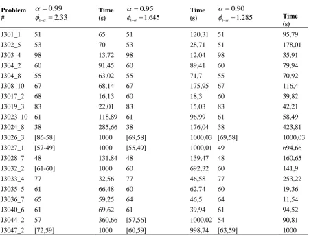
Gurobi 5.0 solver and Python 2.7 interface is used. The 20 deterministic problems are selected randomly, converted to stochastic problems and solved for three different confidence levels
. The time limitation is enforced as 1000 seconds. Results are tabulated at Table 6.
95 . 0
1 1.645
95 . 0
95 . 0
x R1
P N
,
P
xR2
7,1.08
N N
8,1.17
5,0.72
N N
8,1.17
7,1
N N
7,1
9,1.61
N N
7,1.22
7,1.08
N N
7,1.22
95 . 0
25
max
c
k i k
i, 0.2*,
jkMax , Max
j,k
jk
jkk Max Max
R , 3* ,
jk jk
k Max Max
R , 3* ,
0.99,0.95,0.90
,
Table 6. Results of test problems.
Problem #
Time (s)
Time
(s) Time
(s)
J301_1 51 65 51 120,31 51 95,79
J302_5 53 70 53 28,71 51 178,01
J303_4 98 13,72 98 12,04 98 35,91
J304_2 60 91,45 60 89,41 60 79,94
J304_8 55 63,02 55 71,7 55 70,92
J308_10 67 68,14 67 175,95 67 116,4
J3017_2 68 16,13 60 18,3 60 39,82
J3019_3 83 22,01 83 15,03 83 42,21
J3023_10 61 118,89 61 96,99 61 58,49
J3024_8 38 285,66 38 176,04 38 423,81
J3026_3 [86-58] 1000 [69,58] 1000,03 [69,58] 1000,03
J3027_1 [57-49] 1000 [55,49] 1000,01 49 694,66
J3028_7 48 131,84 48 139,47 48 160,65
J3032_2 [61-60] 1000 60 692,32 60 141,9
J3033_4 77 32,56 77 46,58 77 253,22
J3035_5 61 66,48 60 62,74 60 19,36
J3036_7 65 59,25 64 46,5 64 11,54
J3040_6 61 69,62 61 39,94 61 94,52
J3044_2 57 360,66 [57,56] 1000,02 54 90,81
J3047_2 [72,59] 1000 [60,59] 998,74 [63,59] 1000
As can be seen from Table 7, all of the 60 problems are solved within the time limit. However, 10 of them are not optimum. For those problem sets, upper and lower bounds are reported.
4. Conclusion
In this study, stochastic RCPSP was considered with varying resource demands. The deterministic case of the model was further improved with chance constraint, piecewise-linear and mixed integer programming model. The model was tested with known problem instances. One of the main strengths of the model was it can be used as a baseline schedule with a predetermined confidence interval. The proposed model can be used with intelligent based systems in order to model stochastic resource demand conditions, which not only gives an opportunity to modify deterministic models but also increases scheduler’s ability to manage complex project environments. With the rapid developments in computer and information technologies, mathematical programming/modelling-based techniques to solve scheduling problems were significantly receiving attention from researchers. Although it was still not an efficient solution method due to the NP-hard structure of these problems, the mathematical programming formulation was the first Step to develop an effective heuristic. Particularly, for large-scale stochastic RCPSP, the use of heuristics and meta-heuristics methods were inevitable to find good solutions in reasonable time. By using chance constraints, we only guaranteed that the probability of constraints below a predetermined value can be violated but we could not obtain the real cost for violating the constraints. We recommend that in the further research, researchers may develop cost function, which calculates the expected cost of project delay under uncertainty. Developing an effective heuristic on the proposed model increased its effectiveness.
99 . 0
33 . 2
1
10.195.645
90 . 0
285 . 1
1
References
[1] Blazewicz, J., Lenstra, J. K., & Kan, A. R. (1983). Scheduling subject to resource constraints: classification and complexity. Discrete applied mathematics, 5(1), 11-24.
[2] Ballestin, F., & Leus, R. (2009). Resource‐Constrained Project Scheduling for Timely Project Completion with Stochastic Activity Durations. Production and operations management, 18(4), 459-474.
[3] Tavakkoli-Moghaddam, R., Jolai, F., Vaziri, F., Ahmed, P. K., & Azaron, A. (2005). A hybrid method for solving stochastic job shop scheduling problems. Applied mathematics and computation, 170(1), 185-206. [4] Wang, Y., He, Z., Kerkhove, L. P., & Vanhoucke, M. (2017). On the performance of priority rules for the
stochastic resource constrained multi-project scheduling problem. Computers & industrial engineering, 114, 223-234.
[5] Lambrechts, O., Demeulemeester, E., & Herroelen, W. (2008). Proactive and reactive strategies for resource-constrained project scheduling with uncertain resource availabilities. Journal of scheduling, 11(2), 121-136. [6] Valls, V., Laguna, M., Lino, P., Pérez, A., & Quintanilla, S. (1999). Project scheduling with stochastic activity
interruptions. Project scheduling (pp. 333-353). Springer, Boston, MA.
[7] Wang, L., Huang, H., & Ke, H. (2015). Chance-constrained model for RCPSP with uncertain durations. Journal of uncertainty analysis and applications, 3(1), 12.
[8] Uysal, F., Isleyen, S., Cetinkaya, C., & Celik, N. (2015). Resource Constrained Project Scheduling Problem: An Analytical Approach. International conference industrial engineering and environmental protection, 357-362.
[9] Hartmann, S., & Briskorn, D. (2008). A survey of deterministic modeling approaches for project scheduling under resource constraints. European journal of operational research, 207, 1-14.
[10]Kolisch, R., & Sprecher, A. (1997). PSPLIB-a project scheduling problem library: OR software-ORSEP operations research software exchange program. European journal of operational research, 96(1), 205-216. [11]Dadfar, H., & Gustavsson, P. (1992). Competition by effective management of cultural diversity: the case of
international construction projects. International studies of management & organization, 22(4), 81-92. [12]Williams, T. M. (1992). Practical use of distributions in network analysis. Journal of the operational research
society, 43(3), 265-270.
[13]Golenko-Ginzburg, D., & Gonik, A. (1997). Stochastic network project scheduling with non-consumable limited resources. International journal of production economics, 48(1), 29-37.
[14]Shou, Y., & Wang, W. (2012). Robust optimization-based genetic algorithm for project scheduling with stochastic activity durations. International information institute (Tokyo), 15(10), 4049- 4064.
[15]Yang, I. T., & Chang, C. Y. (2005). Stochastic resource-constrained scheduling for repetitive construction projects with uncertain supply of resources and funding. International journal of project management, 23(7), 546-553.
[16] Herroelen, W., & Leus, R. (2005). Project scheduling under uncertainty: Survey and research potentials. European journal of operational research, 165(2), 289-306.
[17]Kis, T. (2005). A branch-and-cut algorithm for scheduling of projects with variable-intensity activities. Mathematical programming, 103(3), 515-539.
[18]Long, L. D., & Ohsato, A. (2008). Fuzzy critical chain method for project scheduling under resource constraints and uncertainty. International journal of project management, 26(6), 688-698.
[19]Schonberger, R. J. (1981). Why projects are “always” late: a rationale based on manual simulation of a PERT/CPM network. Interfaces, 11(5), 66-70.
[20]Golenko-Ginzburg, D., Gonik, A., & Laslo, Z. (2003). Resource constrained scheduling simulation model for alternative stochastic network projects. Mathematics and computers in simulation, 63(2), 105-117.
[21]Li, S., Jia, Y., & Wang, J. (2012). A discrete-event simulation approach with multiple-comparison procedure for stochastic resource-constrained project scheduling. The international journal of advanced manufacturing technology, 63(1-4), 65-76.
[22]Erdogan, S. A., & Denton, B. (2013). Dynamic appointment scheduling of a stochastic server with uncertain demand. Informs journal on computing, 25(1), 116-132.
[23]Charnes, A., & Cooper, W. W. (1959). Chance-constrained programming. Management science, 6(1), 73-79. [24]Charnes, A., & Cooper, W. W. (1962). Chance constraints and normal deviates. Journal of the American
statistical association, 57(297), 134-148.
[25]Charnes, A., & Cooper, W. W. (1963). Deterministic equivalents for optimizing and satisficing under chance constraints. Operations research, 11(1), 18-39.