Fast calculation of the quartet distance between trees of arbitrary degrees

Open Access

Research

Fast calculation of the quartet distance between trees of arbitrary

degrees

Chris Christiansen

, Thomas Mailund*

, Christian NS Pedersen*

,

Martin Randers

and Martin Stig Stissing

Address: 1_{Department of Computer Science, University of Aarhus, Aabogade 34, DK-8200 Århus N, Denmark,} 2_{Department of Statistics, University}

of Oxford, 1 South Parks Road Oxford OX1 3TG, UK and 3_{Bioinformatics Research Center, University of Aarhus, Høegh-Guldbergsgade 10, Bldg.}

090, DK-8000 Århus C, Denmark

Email: Chris Christiansen - [email protected]; Thomas Mailund* - [email protected]; Christian NS Pedersen* - [email protected]; Martin Randers - [email protected]; Martin Stig Stissing - [email protected]

* Corresponding authors

Abstract

Background: A number of algorithms have been developed for calculating the quartet distance between two evolutionary trees on the same set of species. The quartet distance is the number of quartets – sub-trees induced by four leaves – that differs between the trees. Mostly, these algorithms are restricted to work on binary trees, but recently we have developed algorithms that work on trees of arbitrary degree.

Results: We present a fast algorithm for computing the quartet distance between trees of arbitrary degree. Given input trees T and T', the algorithm runs in time O(n + |V|·|V'| min{id, id'}) and space O(n + |V|·|V'|), where n is the number of leaves in the two trees, V and V are the non-leaf nodes in T and T', respectively, and id and id' are the maximal number of non-leaf nodes adjacent to a non-leaf node in T and T', respectively. The fastest algorithms previously published for arbitrary degree trees run in O(n3_{) (independent of the degree of the tree) and O(|V|·|V'|·id·id'), respectively.}

We experimentally compare the algorithm with existing algorithms for computing the quartet distance for general trees.

Conclusion: We present a new algorithm for computing the quartet distance between two trees of arbitrary degree. The new algorithm improves the asymptotic running time for computing the quartet distance, compared to previous methods, and experimental results indicate that the new method also performs significantly better in practice.

Background

The evolutionary relationship for a set of species is con-veniently described by a tree in which the leaves corre-spond to the species, and the internal nodes correcorre-spond to speciation events. The true evolutionary tree for a set of species is rarely known, so inferring it from obtainable

information is of great interest. Many different methods have been developed for this, see e.g. [1] for an overview.

Different methods often yield different inferred trees for the same set of species, and even the same method can give rise to different evolutionary trees for the same set of species when applied to different information about the Published: 25 September 2006

Algorithms for Molecular Biology 2006, 1:16 doi:10.1186/1748-7188-1-16

Received: 18 May 2006 Accepted: 25 September 2006

This article is available from: http://www.almob.org/content/1/1/16

© 2006 Christiansen et al; licensee BioMed Central Ltd.

species. To study such differences in a systematic manner, one must be able to quantify differences between evolu-tionary trees using well-defined and efficient methods.

One approach for comparing evolutionary trees is to define a distance measure between trees and compare two trees by computing this distance. Several distance meas-ures have been proposed, e.g. the symmetric difference metric [2], the nearest-neighbour interchange metric [3], the subtree transfer distance [4], the Robinson and Foulds distance [5], and the quartet distance [6]. Each distance measure has different properties and reflects different aspects of biology.

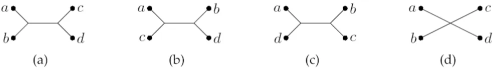
This paper is concerned with calculating the quartet dis-tance. A quartet is a set of four species, the quartet topology

induced by an evolutionary tree is determined by the min-imal topological subtree containing the four species. The four possible quartet topologies of four species are shown in Fig. 1. Given two evolutionary trees on the same set of

n species, the quartet distance between them is the number of sets of four species for which the quartet topologies dif-fer in the two trees.

Steel and Penny [7] pointed at Doucettes unpublished work [8] which presented an algorithm for computing the quartet distance in time O(n3_{), where n is the number of}

species. Bryant et al. in [9] presented an improved algo-rithm which computes the quartet distance in time O(n2₎

for binary trees. Brodal et al. in [10] showed how to com-pute the quartet distance in time O(n log n) considering binary trees. For arbitrary degree trees, the quartet distance can be calculated in time O(n3_{) or O(n}2_d2_{), where d is the}

maximum degree of any node in any of the two trees, as shown by Christiansen et al. [11].

Results and discussion

In [11], we presented an algorithm for computing the quartet distance between trees of arbitrary degree. It runs in time O(n2_d2_{) and space O(n}2_{), where n is the number}

of leaves in each tree and d is the maximal degree found

in either of the trees. In this paper, we present an improved algorithm running in time O(n + |V||V'| min{id, id'}) and space O(n + |V||V'|), where |V| and |V'| are the number of internal (non-leaf) nodes in the two input trees, and id and id' are the maximal degree of an internal node, when disregarding edges to leaves, in the two trees.

Time analysis for different types of trees

The terms |V|, id, |V'| and id' are all clearly O(n), but on the other hand neither |V| and id nor |V'| and id' are inde-pendent. Intuitively, if there are a lot of internal nodes in a tree, they will not have a very large internal degree. We address in this section, how this dependency will affect the running time for different types on trees.

The worst theoretical running time of the algorithm for calculating the quartet distance presented above is O(n3_).

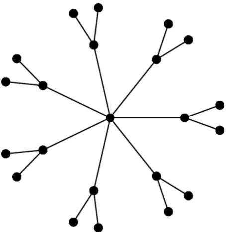
Consider a tree with an internal node of degree ,

con-nected to internal nodes of degree three each

con-nected to two leaves, see Fig. 2. Such a tree has n leaves,

O(n) internal nodes and a maximal internal degree that is

O(n). If the algorithm is run on two such trees, the run-ning time will be O(n3_{). In d-ary trees (trees where all}

internal nodes have degree d) |V| = O ( ), the time

com-plexity of calculating the quartet distance will be O ( ).

The two cases above are somewhat extreme. The first case has a very large gap between the maximal and minimal degree of internal nodes, while the second has little or no gap. The theoretical performance of the algorithm on the two types of trees reflects this difference. Let d_min = min{min_v d_v, min_v' d_v'}, be the minimal degree of any

n

2

n

2

n d

n d

2 The four possible quartet topologies

Figure 1

The four possible quartet topologies. The four possible quartet topologies of species a, b, c, d. Topologies (a): ab|cd, (b):

ac|bd, and (c): ad|bc are butterfly quartets, while topology (d): a , is a star quartet.

b c d

internal node in either tree, then each tree has O( )

internal nodes and the time complexity is O (

min{id, id'}). If min{id, id'} is O( ) the time usage of calculating the quartet distance will be O (n2_{). In the}

fol-lowing section we will do practical verification of the the-oretical results in this section.

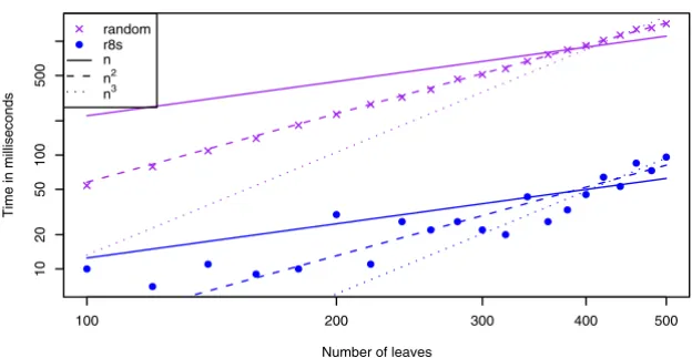
Experimental running times

The graphs in Fig. 3 show the running time for comparing worst case trees (see Fig. 2), (d-ary trees and random trees. There are six types of (d-ary trees; binary, 6-ary, 15-ary, and 30-ary and two types of random trees; r8s-based (see [12]) and trees with random topologies. The trees gener-ated by r8s are binary, but by contracting edges, we can get trees of arbitrary degree (contracting an edge e connecting nodes u and v means removing u and e and attaching the rest of u's edges to v). Each edge is contracted with a prob-ability that is inversely proportional with its length, i.e. a short edge has a higher probability of being contracted than a long edge. The trees with random topology are

gen-erated by adding leaves one by one, starting with a tree of size 2. A leaf can be added by attaching it to a random inner node or by spliting a random edge with a new node, to which the leaf is attached.

The running time for worst case input trees (as described in the previous section) is O(n3_{), because such trees have} O(n) internal nodes and min{id, id'} is O(n). This is sup-ported by the first graph in Fig. 3, which shows that the plot of the polynomial n3 _{(representing the best}

sum-of-squares fit of the polynomial c·n3 _{to the data-points) is}

closest to the plot of the running times with regard to slope.

The running time on the algorithm on d-ary trees is

O( ). The plots of the running times in the second

graph are parallel, and one of them is plotted directly on top of a plot of the polynomial n2 _{(here c·n}2 _{is fitted to the}

data-points for each d separately; the different colors match the d colors). This supports that they all have a run-ning time of O(n2_{) for fixed d's. The graph also shows that}

higher degrees give lower running times, which is also expected. The reason why the algorithm is more than twice as fast on 6-ary trees than it is on binary trees, is that the number of internal nodes in 6-ary trees is less than in binary trees, and even though |V| is O(n) in both cases, that difference has an impact on the running time. The last graph shows the running time of the algorithm on trees created as either random trees (each topology is equally likely) or trees simulated using r8s (with edge contraction as described above). We have no theoretical running time for this data, but the graphs show that the running time is

O(n2_{). Even though the plotted data is only a small}

ran-dom sample, this indicates that many pairs of trees actu-ally have the property that min{id, id'} is O( ). Therefore it is not unreasonable to expect that our algo-rithm runs in time O(n2_{) on trees used in practice. All}

experiments were performed on a standard PC (Pentium 4, 3 GHz, 1 Gb Ram) running Linux Fedora Core 3.

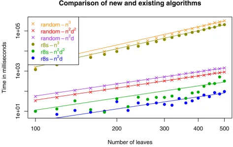
Comparison with existing algorithms

In Fig. 4 we compare the running time of the new algo-rithm with the O(n2_d2_{) and O(n}3_{) time algorithms from}

[11] on random and r8s simulated trees. In Fig. 5 we com-pare the running time of the new algorithm with the other two algorithms on Buneman and refined Buneman trees built for a range of Pfam [13] derived distance matrices using the tool in [14]. Buneman and refined Buneman trees are not binary unless this is well supported by the input distance matrix, and thus represent the kind of trees

n

d_min

n

d

2 2

min

d_min2

n d

2

d_min2 A worst case input tree for the algorithm

Figure 2

A worst case input tree for the algorithm. A tree with an internal node of degree , connected to internal nodes of degree three each connected to two leaves. This tree has both a maximal degree of O(n) and at the same time

O(n) inner nodes.

n

2

n

Experimental running times Figure 3

Experimental running times. The running time of the algorithm for worst case trees, d-ary trees and random trees. The lines plots the polynomials c. ni_{, where c is a fitted constant and i} ∈ _{[1, 4]. The two bottommost plots are in log-scale on both}

the x- and y-axis.

100 200 300 400 500

0

1000

2000

3000

4000

Time usage for the O(n+|V||V'|min{id,id'}) algorithm on worst case trees

Number of leaves

Time in milliseconds

● ● ● ● ● ● ● ● ● ●

● ●

● ●

● ●

● ●

● ●

● ● worst case

n2 n3

n4

100 200 300 400 500

2

5

10

50

200

1000

Time usage for the O(n+|V||V'|min{id,id'}) algorithm on d−ary trees

Number of leaves

Time in milliseconds

● ●

● ●

● ●

● ●

● ● ●

● ● ●

● ● ● ●

● ● ●

● d==3

d==6 d==15 d==30 n n2 n3

100 200 300 400 500

10

20

50

100

500

Time usage for the O(n+|V||V'|min{id,id'}) algorithm on random topology and r8s−based trees

Number of leaves

Time in milliseconds

● ●

●

● ● ●

● ●

● ● ● _● ●

● ●

● ●

● ●

● ● ●

which can only be compared by methods which allow for trees of arbitrary degrees. In both experiments, the O(n3₎

time algorithm is slowest by a large margin for all plotted sizes of n. The new algorithm is consistently faster than the O(n2_d2_{) time algorithm for the r8s (with edge}

contrac-tion) simulated trees and for the Buneman and refined Buneman trees. For random trees the previous O(n2_d2₎

time algorithm is slightly faster in practice. This difference is most likely caused by the additional overhead of precomputing the sums used by the new O(n2_{d) time}

algorithm compared to the previous O(n2_d2_{) time}

algo-rithm in order to improve the asymptotic worst case run-ning time (see method section). For trees of low degree, the overhead might dominate the factor d by which the worst case running time of the new algorithm is improved. The observed running times on random trees thus indicate that over selection of random trees consists of trees of low degree, whereas the r8s simulated, Bune-man, and refined Buneman trees are trees with a few

nodes of high degree which more than compensate for the additional overhead of dealing with nodes of low degree. In conclusion, we find that the experimental comparison of the new algorithm with the previously developed algo-rithms indicate that the new algorithm not only improves on the theoretical asymptotic running time, but also improves the running time in practice if the input trees contain a few nodes of high degree.

Conclusion

We have constructed an algorithm for finding the quartet distance between two trees of arbitrary degree. It runs in time O(n + |V||V'| min{id, id'}) and uses space O(n + |V||V'|), where n is the number of leaves in the trees, |V| and |V'| are the number of internal nodes in the trees and

id and id' are the maximal internal degree of internal nodes in input tree T and T' respectively. Internal degree of an internal node is the number of internal nodes

con-Comparisons with earlier algorithms on random and r8s trees Figure 4

Comparisons with earlier algorithms on random and r8s trees. The running time for the new algorithm compared to the existing O(n2_d2_{) and O(n}3_{) time algorithms for random and r8s trees. The lines are fitted polynomial c. n}2_{, for the case of the}

new algorithm (denoted n2_{d in the legend) and the O(n}2_d2_{) algorithm, and the polynomial c. n}3 _{for the O(n}3_{) algorithm. The plot}

is in log-scale on both the x- and y-axis.

100

200

300

400

500

1e+01

1e+03

1e+05

Comparison of new and existing algorithms

Number of leaves

Time in milliseconds

●

● ● ● ●

●

●

● _● ● _{● ●} ● ● ●

● ● ● ● ● ●

● ●

●

● ●

●

●

● _● ● ● ●

●

● ● ●

● ● ● ●

● ●

● ●

● ●

● ●

● ● ●

● ● ●

● ● ● ●

● ● ● ●

● ● ●

random

−−

n

random

−−

n

d

random

−−

n

d

r8s

−−

n

r8s

−−

n

d

nected to it, so neighbouring leaves do not add to this value. The values |V|, |V'|, id and id' are not independent, therefore we have investigated how the structure of the trees affect the running time of the algorithm. We show that the time used to count the butterfly quartets – topol-ogies where one pair of the four leaves is separated from the other pair by an edge – is reduced to O(n2_{) when}

min{id, id'} = O( ), where d_min is the minimal degree of all internal nodes in the trees. If the input trees are d -ary, that is all internal nodes have degree d, the running

time is O( ), excluding the time to find intersections.

These theoretical running times have been validated by running a series of tests using a Java implementation of the algorithm, available at [15]. We also done a series of tests on random trees, trees generated by the program r8s, Buneman trees, and refined Buneman trees. Running the algorithm on these trees gives an impression on how it

performs on trees used in practice. On both types of trees the running time appears to be O(n2_{). It is however still an}

open problem to develop an algorithm running in time

O(n2_{)for all types of trees.}

Methods

Consider two input trees, and assume that a quartet has butterfly topology in both trees, i.e. that one pair of the four leaves is separated from the other pair by an edge in the tree in both trees. We say that the butterfly quartet is

shared, if it has the same butterfly topology in both trees. Otherwise, we say that the butterfly quartet is nonshared. We let shared(T, T') denote the number of butterflies shared between tree T and tree T', i.e. the number of quar-tets that are butterflies with the same topology in tree T

and tree T', and let nonshared (T, T') denote the number of quartets that are butterflies in both T and T' but with different topology. By our definition of shared, the number of butterfly quartets in a single tree can be stated as the number of butterfly quartets shared between the

d_min2

n d

2

Comparisons with earlier algorithms on Buneman and refined Buneman trees Figure 5

Comparisons with earlier algorithms on Buneman and refined Buneman trees. The running time for the new

O(n2_{d) time algorithm compared to the existing O(n}2_d2_{) and O(n}3_{) time algorithms on the Buneman and the refined Buneman}

trees for range of Pfam based distance matrices. The plot is in log-scale on both the x- and y-axis.

● ● ●● ●●●● ● ●● ●●●● ●●● ● ● ● _● ●_●●●● ● ●● ● ● ● ● ● ● ● ● ● ● ● ●● ● ● ● ● ●● ●● ● ● ●●●●● ● ● ● ● ● ● ● ● ● ●● ● ● ● ● ● ● ● ●● ● ● ● ● ● ● ● ● ● ● ● ● ● ● ● ● ● ● ● ● ● ● ● ● ● ● ● ●● ● ● ●● ●●● ● ●● ● ●●● ● ● ●●

10

20

50

100

200

500

1000

5e−01

5e+00

5e+01

5e+02

Comparison on Buneman and refined Buneman trees

Number of leaves

Time (in sec)

● ● ●● ●●●● ● ●● ●●●● ●●● ● ● ● ● ●●●●● ● ●● ●● ●●● ● ● ●● ● ● ●● ● ● ● ● ●● ●● ●●●●●● ● ● ● ● ● ●● ● ● ● ●● ● ● ● ●●● ● ●● ● ● ● ● ● ● ● ● ● ● ● ● ● ● ● ● ● ● ● ● ● ● ● ● ● ● ● ● ● ● _● ● ● ● ● ● ● ●● ● ●● ● ● ● ●● ● ● ●● ● ● ● ● ● ● ● ● ●_● ● ● ●● ● ● ● ● ●● ● ● ● ● _{● ●} ● ● ● ● ● ● ●●● ● ● ●● ● ● ● ● ●● ●● ● ● ● ● ●● ● ● ● ● ● ● ● ● ● ● ●● ● ● ● ● ● ● ● ● ● ● ● ● ● ● ● ● ● ● ● ●●● ● ● ● ● ● ● ● ● ● ● ● ● ● ● ●● ● ● ●●●●●●●●●●●●●●●●

tree and itself, i.e. shared(T, T) or shared(T', T') for the number of butterfly quartets in T and T' respectively. (This notation also emphasizes that computing the number of butterfly quartets in a single tree by our algorithm is per-formed as a comparison of the tree against itself.)

In [11] we argue that the quartet distance between T and

T', qdist(T, T'), can be found by focusing only on the com-putation of the number of shared and nonshared butterfly quartets between two trees, i.e. it is unnecessary to con-sider non-butterfly quartets explicitely. More specifically, we show that:

The proof of this formula is a follows. Let Q denote the number of quartets which have butterfly topology in T

and non-butterfly topology in T'. Symmetrically, let Q'

denote the number of quartets which have butterfly topol-ogy in T' and non-butterfly topology in T. A butterfly quartet in T is either a butterfly quartet in T' or a non-but-terfly quartet in T'. The number of butterfly quartets in T, shared(T, T), can thus be expressed as the sum shared(T,

T') + nonshared(T, T') + Q. Similarly, the sum shared (T',

T') = Q' + shared (T, T') + nonshared (T, T'). It is now straightforward to verify that the righthand side of (1) adds up Q + Q' + nonshared(T, T') which is the number of quartets where the quartet topologies differ in T and T', i.e. qdist(T,T').

In the section below, we describe how to use (1) to com-pute the quartet distance in time O(n + |V||V'| min{id,

id'}), more precisely O(n + |V||V'|) for a preprocessing step, after which we can use O(|V||V'|) for calculating shared(T, T'), O(|V||V'|{id, id'}) for calculating non-shared(T,T'), O(|V|) for calculating shared(T,T) and

O(|V'|) for calculating shared(T',T').

Terminology

Let T and T' be two unrooted trees. In this paper we will explicitly refer to the leaves of a tree as leaves and the non-leaf nodes as internal node. We will assume that T and T'

each has n labelled leaves numbered 1,..., n such that the leaf numbered x in T has the same label as the leaf num-bered x in T'. The leaf sets are denoted L and L' for T and

T' respectively, note that L = L'. We will use V and V' to denote the internal nodes in T and T' respectively. The

degree of an internal node v is the number of subtrees con-nected to it, and is denoted d_v. The internal degree of an internal node v, id_v, is the number of non-leaf subtrees connected to it. We will assume that no internal node in T

and T' has degree two, and we will denote the maximal internal degree of all internal nodes in T and T' by id and

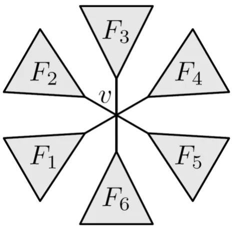
id' respectively. Let v be an internal node in T, and let F₁, ..., be the subtrees connected to it, as shown in Fig. 6

We call these the subtrees of v. We say that v claims all but-terfly quartets ab|cd where a,b ∈F_i, c ∈F_k and d ∈F_m for i

≠k ≠ m (see Fig. 7). With this definition, each butterfly quartet is claimed by exactly two internal nodes.

Adding the subscript yz|w|x to an internal node claiming the butterfly quartet wx|yz, indicates that the leaves y and

z are found in a single subtree of the internal node, while the leaves w and x are found in different subtrees. For example, considering the quartet ab|cd, v and v' in Fig. 7 are written as vab|c|d and .

Given a subtree F of T, and a subtree G of T', we call the intersection F ∩G a shared leaf set, i.e. the set of leaves present in both F and G. The size of the shared leaf set, |F

∩G|, then denotes the number of leaves present in both F

and G. The size of a single subtree F is similarly denoted |F|. We will use to represent the subtree of T containing all leaves not in F and similarly for and G in T', see Fig. 8 for an example. Note that and are also subtrees of

T and T' respectively, and thus |F ∩G|, | ∩G|, |F ∩ | and | ∩ | are all sizes of shared leaf sets between a sin-gle subtree from T and a single subtree from T'. In the

pres-qdist shared shared

shared nons

( , ) ( , ) ( , )

( , )

T T T T T T

T T

′ = + ′ ′

− ⋅2 ′ − hhared( , )T T′ ( )1

F_d

v

′

v_{ab c d| |}

F

G

F G

F G

F G

An internal node v ∈T with subtrees F1,...,Fd, here dv = 6

Figure 6

entation of the algorithms below, we will assume that we have access to |F|, |G| and |F ∩G| for all subtrees F of T

and G of T' in time O(1). At the end of the section we will describe how this can be achieved by an O(n) time pre-processing step, which does not affect the asymptotic worst case running time of the presented algorithms.

Counting shared butterfly quartets

For each pair of internal nodes v, v' from T, T' we want to count the number of shared butterfly quartets claimed by both internal nodes, shared(v, v'). Assume that F₁, ...,

are subtrees of v and G₁, ..., are subtrees of v'. We wish

to count all quartets on the form ab|cd where a, b ∈F_i ∩ G_j, c ∈F_k ∩G_l and d ∈F_m ∩G_n, i ≠k ≠m, j ≠l ≠n (see Fig. 7). Counting the possible combinations of a and b is expressed by the following double sum, which sums over all pairs of subtrees of v and v':

Given that a and b are in F_i ∩G_j, we need to find c and d

in _i ∩ _j. The number of possible choices of c and d is expressed by:

However when finding c and d in i ∩ j, the condition

that c and d must be in different subtrees is not satisfied. Therefore we subtract the number of times c and d are in the same subtree of v and v':

Any pair in F_k ∩G_l is counted twice, once in |F_k ∩ _j| and once in | _i ∩G_l|, therefore these pairs are subtracted once using the double sum above. (2) expresses the number of ways c and d can be found in different subtrees, given that a and b are found in F_i ∩G_j:

F_d

v

G_d

v′

|F_i G_j| j

i

∩  

 _

∑

∑

F G

|F_i∩G_j|

 

 ₂ _

F G

|F_k G_j| |F_i G_l| |F G | l j

k i

k l

l j

∩  

 _ + _ ∩  

 −  ∩ 

 

 

≠

≠

∑

∑

∑

kk i

∑

G

F

|Fi Gj| |Fk Gj| |F G| |

k i

i l

l j

∩  

 _ − _ ∩ _ − _ ∩    +

≠ ≠

∑ ∑

2 2 2

F Fk Gl l j k i

∩    



 ( ) ≠

≠∑

∑ 2 | 2

A rooted subtree F, and its complement rooted subtree

Figure 8

A rooted subtree F, and its complement rooted subtree .

F F

Internal nodes v ∈T and v' ∈T', each claiming the quartet ab|cd

Figure 7

We can now compute the number of shared butterfly quartets between two internal nodes, ie. the number of butterfly quartets claimed by both internal nodes with the same topology:

If the trees, T and T', have a shared quartet ab|cd, then there are two internal nodes in each tree that claims this quartet: v_ab|c|d and v_cd|a|b in T and and in T'. Since both shared(v_ab|c|d, ) and shared(v_cd|a|b, ) will count the quartet, the total number of shared quartets between the two trees is:

It is straightforward to observe that calculating shared(v,

v') using a direct computation of (3) takes time O( ). It is however not necessary for shared(v, v') to sum over all subtrees of v and v'. Since each term in the sums involves taking a 2-subset from a shared leaf set, we need only to consider subtrees that are not leaves. This reduces the run-ning time to O( ). This running time can be improved even more, we start by expressing (2) in a differ-ent way:

Let

We can ignore leaf subtrees, so we need to compute id_v'

different _j's and S_j's which can each be computed in

O(id_v) time. Symmetrically each of the id_v 's and 's takes time O( ) to compute, and the total time of com-puting S is O(idvidv'). The total time of computing all sums

mentioned is thus O(id_vid_v') and this is the key to reducing the time usage of shared(v,v'). Using the sums we can express (4) as:

Provided that the sums _j, , S_j, and S have been cal-culated, (4) can be calculated in time O(l). Since calcula-tion of the sums is independent on the calculacalcula-tion of shared(v, v'), these calculations can be done serially as shown in the algorithm below, thereby reducing the time usage of shared(T, T') to:

ALGORITHM – CALCULATING THE NUMBER OF SHARED BUTTERFLY QUARTETS BETWEEN T AND T'

Requires: T, T' two input trees with the same leaf set.

Ensures: Res = shared(T, T')

Res ← 0

for v internal node in T do

for v' internal node in T' do

shared v v Fi Gj F G F G

j i

i j k j

, ′ | | | | | | ( )=  ∩   _  ∩   _ − ∩ ∑

∑ _{2 2}  ₂

  _     −  ∩      +  ∩      ≠ ≠ ≠ ≠ ∑ ∑ ∑ k i

i l k l

l j k i l j

F G F G

| | | | 2 2 ∑ ∑    

( )3

′

vab c d| | v′cd a b| |

′

v_{ab c d| |} v′_{cd a b| |}

shared( , )T T shared( , )v v

v T v T ′ = ′ ′∈ ′ ∈

∑

∑

d d_{v v}2 2_′

id id_v2 _v2_′

|Fi Gj| |F G| |F

I k j k i II i ∩    _ − _ ∩ _ − ≠ ∑ 2 2 ∩ ∩       +  ∩      ≠ ≠ ≠

∑ Gl ∑∑ F G

l j III k l l j k i IV | | | 2 2 = ∩  

|Fi Gj|_ − _|F ∩G| +_ _|F∩G|

I

k j i j

2 2 2

   − _ ∩    + ∩   _ ∑ ∑ k II

i l i j

l

II

F G F G

| | | | 2 2 II k l l k k j k i

F G F G F

+  ∩      −  ∩   _ − ∩ ∑

∑ | 2 | ∑ | 2 | | G

G_l Fi Gj l IV | | | 2 2       + ∩   _ ∑ 4 ( )

S F G

S F G

S F G

j

k j

k

i i l

l

j k j

=  ∩   _ ′ =  ∩      =  ∩   _

∑

∑

∑

∑

∑

∑

i i l

l

k l

l k

S F G

S F G

| | | | 2 2 5 S ′

S_i S_i′

id_v′

|F G | | |

S F G S

i j

I

j i j

II

∩  

 ₂ _ − +_ ∩₂ _ − ′

ii i j

III

j i

i j

I

F G

S S S F G

+ ∩ 

| ₂ |_ + − − ′ + _| ∩₂ |_

V V

S S_i′ S_i′

id id_{v v} id id V V O V V

v T v v T v v T ′ ′∈ ′ ∈ ′∈ ′ ′

∑

∑ ∑

Calculate sums _j, , S_j, and S

Res ←Res + shared(v, v')

end for

end for

Res ←

Counting nonshared butterfly quartets

For each pair of internal nodes v, v' we want to count the number of nonshared butterfly quartets claimed by both internal nodes, nonshared(v, v'). Such quartets have the property that a pair of leaves found in the same subtree of

v will be found in different subtrees of v' and vice versa, i.e. a nonshared quartet with leaves a, b, c and d, has a ∈F_i ∩ G_j, b ∈F_i ∩G_l, c ∈F_k ∩G_n and d ∈F_m ∩G_j (see Fig. 9). The following expression counts all nonshared quartets related to a pair of nodes v and v', obeying that if two leaves of the quartet are in one subtree of v they are in dif-ferent subtrees of v' and vice versa:

Even though (6) satisfies the property of nonshared quar-tets, it possibly counts more than the number of non-shared quartets claimed by an internal node in each tree. The problem is that given two internal nodes, they do not nescessarily claim the quartets counted by (6). If we

denote the leaves of an nonshared quartet a, b, c and d, the first, second, third and fourth factors in (6) counts the number of choices of a, b, c and d respectively. The first and second factor choose a and b from F_i, while the third and fourth choose c and d from _i. In the cases where c

and d are chosen from the same subtree F_k, k ≠i of v, v does not claim the quartet. We must subtract these quartets, which can be counted as:

Similarly there are cases where b and c are chosen from the same subtree G_l, l ≠j of v', which we must also subtract. These can be counted as:

The cases where both c and d are chosen from the same subtree F_k, k ≠i of v and b and c are chosen from the same subtree G_l, l ≠j of v' are included in both the expressions above and therefore they must be added again. The fol-lowing expression counts the number of these cases:

Combining equations (6), (7), (8) and (9), gives a way of calculating the number of nonshared quartets between two internal nodes v and v':

S S_i′ S_i′

Res

2

|Fi Gj||Fi Gj||Fi Gj||Fi Gj|

j i

∩ ∩ ∩ ∩ ( )

∑

∑

F

|F_i G_j||F_i G_j||F_k G_j||F_k G_j| k i

j i

∩ ∩ ∩ ∩ ( )

≠

∑

∑

∑

|Fi Gj||Fi Gl||Fi Gl||Fi Gj|

l j j i

∩ ∩ ∩ ∩ ( )

≠

∑

∑

∑

|Fi Gj||Fi Gl||Fk Gl||Fk Gj|

l j k i j i

∩ ∩ ∩ ∩ ( )

≠ ≠

∑

∑

∑

∑

Internal nodes v ∈T claiming the quartet ab|cd and v' ∈T' claiming the quartet ad|bc

Figure 9

Assuming that the trees have a nonshared quartet with topology form ab|cd in T, and ad|bc in T', there are two internal nodes in each tree claiming the quartet: v_ab|c|d and

v_cd|a|b in T and and in T'. All of the four com-binations of these will identify the quartet as nonshared. Therefore the total number of nonshared quartets between the two trees is:

Direct computation of nonshared(v, v') using (10) takes

time O( ). Each of the subtrees has to be intersected with two disjoint sets in each of the sums. This means that if a subtree is only a leaf, at least one of these intersections will be zero, and the term will be zero. Therefore we can ignore subtrees that consist of a single leaf, just like when computing shared(T, T'), and reduce the time usage to

O( ). The time usage of the calculation of non-shared(v, v') can be further improved by rewriting (9):

Inspired by the precomputing of sums used in shared(v,

v'), (5), we calculate for each i, k, k ≠i the sum:

There are O( ) of these sums and each takes time

O(id_v') to calculate, so the time complexity for calculating

all sums is O( ). In the case that idv' ≤idv, we can

switch v and v' and thus get time usage O(id_vid_v' min{id_v,

id_v'}). Assuming that the sums have been calculated, (9) can now be calculated in time O(idvidv'min{idv, idv'}) by

the expression:

By substituting (9) with (12) in (10), we can calculate nonshared(v, v', in time O(id_vid_v'min{id_v, id_v'}). Since cal-culation of the sums is independent of the calcal-culation of nonshared(v, v'), these calculations can be done serially as shown in the algorithm below.

ALGORITHM – CALCULATING THE NUMBER OF NON-SHARED BUTTERFLY QUARTETS BETWEEN T AND T'

Requires: T, T' two input trees with the same leaf set.

Ensures: Res = nonshared(T, T')

Res ← 0

for v internal node in T do

for v' internal node in T' do

Calculate sums Si,k

Res ←Res + nonshared(v, v')

end for

end for

Res ←

The time complexity of the algorithm is:

Counting butterfly quartets in a single tree

Reusing the idea of precomputing certain sums enables us to calculate the number of butterfly quartets in a single tree T in time O(|V|). Since the number of butterfly quar-tets in a single tree is the number of butterfly quarquar-tets shared between the tree and itself, we will use shared(T, T) to denote the number of butterfly quartet in T. This nota-tion also emphasizes that computing the number is essen-tially a comparison of the tree against itself. Given a node

v in T we can express the number of quartets it claims in the following way:

where the F_i's are the subtrees of v. Now let

nonshared(v,v′)= ( ∩ ∩ ∩ ∩

− ∩

∑

∑ | || || || | | ||

F G F G F G F G

F G

i j i j i j i j

j i

i j FF G F G F G

F G F G F G F G

i j k j k j

k i

i j i l i l i j

l j ∩ ∩ ∩ −≠ ∩ ∩ ∩ ∩ ≠ ∑ ∑ || || | | || || || | ++ ∩ ∩ ∩ ∩   ( ) ≠ ≠∑

∑ |Fi Gj||Fi Gl||Fk Gl||Fk Gj|

l j k i

10

′

v_{ad b c| |} v_{bc a d}′_{| |}

nonshared( , )T T nonshared( , )v v

v T v T ′ = ′ ′∈ ′ ∈

∑

∑

d d_{v v}2 2_′

id id_v2 _v2_′

| || || || |

| | |

F G F G F G F G

F G F G

i j i l k l k j l j k i j i i j j i k j ∩ ∩ ∩ ∩ = ∩ ∩ ≠ ≠

∑

∑

∑

∑

∑

∑

i l k l l j i j j i k j k i

i l k

F G F G

F G F G F G F

≠ ≠ ≠

∑

∑

∑

∑

∑

∩ ∩ ∩ ∩GG_l F G F G

l

i j k j

| | || |

∑



 

S_{i k} F_i G_l F G

l

k l

, =

∑

id_v2

id id_v2 _v′

|Fi Gj| |F G | S, |F G ||F G |

j i

k j i k i j k j k i ∩ ∩

(

)

∑

∑

∑

id idv v′min{id idv, v′}≤min{id id, ′} idv idv′=O V(| ||V′| min{id id, ′}})

′∈ ′ ∈ ′∈ ′ ∈ ∑ ∑ ∑ ∑ v T v T v T v T

F_i F_i F_j

j i

i 2 2 2

we can now express (13) as

S can be calculated in time O(idv)and using the

precom-puted S, (14) can be also calculated in time O(id_v). Sum-ming the results of (14) for all nodes in T gives the number of quartets in the tree, shared(T, T). The total time usage is

Calculating the shared leaf set sizes

The algorithms presented above all rely on O(1) time access to the size of the shared leaf set |F ∩G| for any pair of subtrees F of T and G of T', where F and G each has size at least two, i.e. contains more than a single leaf. We will refer to |F ∩G| as the intersection size of subtree F and G. In [9] and O(n2_{) time and space algorithm is presented for}

computing the intersection sizes of all pairs of subtrees F

and G of two binary input trees. A straightforward gener-alization of this algorithm to two input trees T and T' of arbitrary degrees results in an O(n2_{dd') time and O(n}2₎

space algorithm, which gives a worst case running time of

O(n4_).

In this section we will present an improved algorithm for computing the intersection sizes of all pairs of subtrees of

T and T' which runs in time O(n + |V||V'|) and space

O(|V||V'|). We will assume that the size of each subtree F

of T and G of T', i.e. |F| and |G|, is available in time O(1). This can be achieved as presented in the next section. Our algorithm for computing all intersection sizes is as fol-lows. Choose an arbitrary node r in T and an arbitrary node r' in T'. Rooting the trees in r and r' respectively gives rise to two rooted trees T_r and , Fig. 10 shows an exam-ple of rooting a tree. Calculating the shared leaf set sizes of Tr and and all subtrees in both trees can be done

using:

where Fi are all subtrees of Tr and Gj are all subtrees of .

This can be calculated using dynamic programming in time O(n2_):

Except |T_r ∩ |, the shared leafset sizes calculated by (15) are the shared leaf set sizes of all rooted subtrees of T and

T' that do not contain the nodes r and r'. Assuming that the subtree F of T does not contain r, then the subtree

does contain r and similarly for r' and subtrees G and of T'. The shared leaf set sizes of these trees that do contain

r and r' can be calculated from the intersection sizes that we have available using (16):

S Fj

j

=    _

∑

F F

S F

i i i

i 2 2 2

14

   

  

  

  − +

  

  



 _⋅ ( )

∑

id_v O V

v T

∑

=

(

)

′

T_r

′

T_r

|T_r T_r| |F_i G_j| |F_i G| |F G_j|,

j i

j i

∩ ′ =

∑

∑

∑

∑

′

T_r

d d_{v v} d_v d_{v O n}

v V

l L l Ll L

l L v V v V

v

′ ′

′∈ ′

∈ ∈ ′∈ ′

′∈ ′ ∈ ′∈ ′

∈

+

∑

∑

∑

∑

∑

∑

( )

∑

V V

∑

′

T_r

F G

An arbitrary node, r, is chosen as the root in the tree, leading to a rooted tree

Figure 10

In other words all shared leaf set sizes can be calculated in time O(n2_{). First the shared leaf set sizes for subtrees that}

to not contain an arbitrary node r and r' from each tree are calculated in time O(n2_{). Then the shared leaf set sizes of}

subtrees that do contain r or r' (or both) are calculated constant time for each shared leaf set. Since there are

O(n2_{) shared leaf sets the total time usage is O(n}2_).

The reduction to time O(n + |V||V'|) and space O(|V||V'|) is done by handling the cases where F, Fi, G or Gj is a leaf

in a special way. For each pair of nodes v, v' we let Leaf [v,

v'] be the number of leaves directly connected to v that have the same label as a leaf directly connected to v'. Leaf

[v, v'] is constructable in time O(n + |V|||V'|) in the follow-ing way: First, set Leaf [v, v'] = 0 for all pairs of nodes v, v'. Given a leaf number, x, there is a unique node, node(x), in

T and a unique node, node'(x), in T'. For each leaf number,

x, we increment Leaf [node(x), node'(x)]. There are n such numbers, and by assumption, the leaves can be found in constant time given a number. Thus Leaf [v, v'] is con-structable in time O(n + |V||V'|). We choose r and r' in T

and T' and create two rooted trees T_r and . The non-leaf

children of r in T_r are F₁,..., F_x and the non-leaf children of

r' in are G1,..., Gy. The intersection size of the two trees

can be defined recursively as:

The first term counts all leaves directly connected to both

r and r'. The second term counts all leaves connected directly to r', that are also in T_r, but not directly connected to r. The third term counts all leaves connected directly to

r, that are also in , but not directly connected to r'. Sum-ming these three terms counts all leaves present in both subtrees, but leaves not connected directly to the roots are counted twice, and are subtracted by the last term.

Since (17) is only summing over the non-leaf children of a given internal node, calculating the shared leaf set sizes of all these pairs of subtrees can be done using dynamic pro-gramming in time:

By the same arguments as above, the rest of the shared leaf set sizes can be computed in time O(|V||V'|) and space

O(|V||V'|). Therefore the total running time of the algo-rithm is O(n + |V||V'|) and space usage is O(|V||V'|).

Calculating the sizes of all subtree leaf sets

All of the above algorithms make use of the sizes of the leaf sets of the rooted subtrees of the input trees, either directly or indirectly. Rooting T in an arbitrary node r

gives rise to the rooted tree T_r. Every subtree F_x of T_r is a rooted subtree of T, and _x is also a rooted subtree of T. Note that the set of subtrees Fx ∪ x, since one tree is the

complement of the other, contains all subtrees of T and that | _x| = n - |F_x|. By using dynamic programming the sizes of all subtrees, F_x, can be computed by a single traver-sal of T_r. For each F_x the size of _x can be computed in constant time, since n is known. This means that all leaf set sizes of a tree of arbitrary degree can be calculated in time O(n).

Authors' contributions

All authors participated in developing the algorithm. CC and MR implemented the algorithm and conducted the experiments. All authors participated in drafting of the manuscript.

References

1. Felsenstein J: Inferring Phylogenies Sinauer Associates Inc; 2004. 2. Robinson DP, Foulds LR: Comparison of weighted labelled

trees. In Combinatorial mathematics, VI (Proc 6th Austral Conf) Lecture Notes in Mathematics, Springer; 1979:119-126.

3. Waterman MS, Smith TF: On the similarity of dendrograms.

Journal of Theoretical Biology 1978, 73:789-800.

4. Allen BL, Steel M: Subtree transfer operations and their induced metrics on evolutionary trees. Annals of Combinatorics 2001, 5:1-13.

5. Robinson DP, Foulds LR: Comparison of phylogenetic trees.

Mathematical Biosciences 1981, 53:131-147.

6. Estabrook G, McMorris F, Meacham C: Comparison of undirected phylogenetic trees based on subtrees of four evolutionary units. Syst Zool 1985, 34:193-200.

7. Steel M, Penny D: Distribution of tree comparison metrics– some new results. Syst Biol 1993, 42(2):126-141.

8. Doucette CR: An Efficient Algorithm to Compute Quartet Dissimilarity Measures. 1985. [Unpublished, Bachelor of Science (Honours) Dissertation. Memorial University of Newfoundland] 9. Bryant D, Tsang J, Kearney PE, Li M: Computing the quartet

dis-tance between evolutionary trees. Proceedings of the 11th Annual Symposium on Discrete Algorithms (SODA) 2000:285-286.

10. Brodal GS, Fagerberg R, Pedersen CNS: Computing the Quartet Distance Between Evolutionary Trees in Time O(n log n).

Algorithmica 2003, 38:377-395.

11. Christiansen C, Mailund T, Pedersen CNS, Randers M: Computing the Quartet Distance Between Trees of Arbitrary Degree.

In Proceedings of Workshop on Algorithms in Bioinformatics (WABI) Vol-ume 3692. LNBI, Springer-Verlag; 2005:77-88.

12. r8s [http://ginger.ucdavis.edu/r8s/]

13. Pfam [http://www.sanger.ac.uk/Software/Pfam/]

14. Besenbacher S, Mailund T, Westh-Nielsen L, Pedersen CNS: RBT – A tool for building refined Buneman trees. Bioinformatics 2005,

21:1711-1712.

15. QuartetDist [http://www.daimi.au.dk/~chrisc/qdist/]

| | | | | |

| | | | | |

| | | | | | | |

F G G F G

F G F F G

F G n G F F G

∩ = − ∩

∩ = − ∩

∩ = −

(

)

( )16

′

T_r

′

T_r

|Tr Tr| Leaf r r, |Fi Tr| |T G | |F G | i

x

r j i j

j y

i x

∩ ′ = [ ′]+ ∩ ′ + ∩ − ∩

= = =

∑ ∑

1 ∑j= ∑∑1 1 ( )

y

1

17

′

T_r

n V V id_v id_v id id O n V V

v V

v v v V v V v

+ ′

(

)

(

)

′∈ ′ ∈ ′∈ ′ ′

∑

∑

∑

| || | | || |

∈ ∈

∑

V

F

F

F