Type of the Paper (Article)
1
Bayesian Bias Correction of Satellite Rainfall
2
Estimates for Climate Studies
3
Margaret Wambui Kimani 1, Joost C.B. Hoedjes 1, Zhongbo Su 1
4
1 Faculty of Geo-Information Science and Earth Observation, University of Twente, Enschede, 217 7500 AE,
5
Netherlands
6
Correspondence to: Margaret W. Kimani ([email protected])
7
8
Abstract: Advances in remote sensing have led to use of satellite-derived rainfall products to
9
complement the sparse rain gauge data. Although globally derived and some regional bias
10
corrected, these products often show large discrepancies with ground measurements attributed to
11
local and external factors that require systematic consideration. Decreasing rain gauge network
12
however inhibits continuous validation of these products. We propose to deal with this problem by
13
the use of Bayesian approach to merge the existing historical rain gauge information to create a
14
consistent satellite rainfall data that can be used for climate studies. Monthly Bayesian bias
15
correction is applied to the Climate Hazards Group Infrared Precipitation with Stations (CHIRPS
16
v2) data to reduce systematic errors using a corresponding gridded (0.05°) rain gauge data over East
17
Africa for a period of 33 (1981–2013) years of which 22 years are utilized to derive error fields which
18
are then applied to an independent CHIRPS data for 11 years for validation. The bias correction is
19
spatially and temporally assessed during the rainfall wet months of March-May (MAM),
June-20
August (JJA) and October–December (OND) in East Africa. Results show significant reduction of
21
systematic errors at both monthly and yearly scales and harmonization of their cumulative
22
distributions. Monthly statistics showed a reduction of RMSD (29–56)% and MAE (28–60)% and an
23
increase of correlations (2–32) %, while yearly ones showed reductions of RMSD (9-23)%, and MAE
24
(7–27)% and increase of correlations (4–77)% for MAM months, reduction of RMSD (15–35)% and
25
MAE (16–41)% and increase in correlations (5–16)% for JJA months, and reduction of RMSD (3–35)%
26
and MAE (9–32)% and increase of correlations (3–65)% for OND months. Systematic errors of
27
corrected data were influenced by local processes especially over Lake Victoria and high elevated
28
areas. Large-scale circulations induced errors were mainly during JJA and OND rainfall seasons and
29
were reduced by the separation of anomalous years during training. The proposed approach is
30
recommended for generating long-term data for climate studies where consistencies of errors can
31
be assumed.
32
Keywords: Bayesian bias correction; satellite rainfall; rain gauge; climate studies; East Africa
33
34
1. Introduction
35
High temporal and spatial rainfall distribution is vital for many applications such as climate
36
studies, water resource management and agriculture. Rain gauges provide the most direct
37
representations of rainfall, but their distribution over land is sparse, especially in mountainous
38
areas [1], and being point observations, they lack spatial representativeness. Use of satellite rainfall
39
products is increasing because of their high spatiotemporal coverage. However, these products
40
often exhibit large discrepancies with ground measurements [2,3] and the errors need to be reduced
41
to make the products more representative of the rainfall variability. This has been done at global
42
scale (Krajewski et al., 2000; Huffman et al., 2007; Arkin and Xie, 1994) and some regional
43
evaluations [4,5], but relatively few efforts have been made to reduce the often large errors that
44
occur at local scales. Studies have found that satellite rainfall products have systematic errors that
45
cause overestimations/ underestimations [6] [7,8], especially on high elevated areas.
46
Different bias correction approaches for improving the satellite rainfall estimates have been
47
proposed. [7] applied bias correction using empirical cumulative distribution (CDF) maps on a
48
seasonal basis for hydrological applications in the upper Blue Nile in Ethiopia. The choice of the
49
seasonal scale was meant to reduce error related to temporal variability but in areas of high rainfall
50
variabilities, seasonal scale may not capture such variabilities. It is worth noting that effectiveness
51
of bias correction of rainfall products may differ from location to location and consideration of
52
spatial scale is of great importance. This was observed by [9,10] who used of quantile mapping
53
approach to bias correct model rainfall products and observed that the approach improves the
54
estimates in some locations, while it degrades in others.
55
[9] assessed the performance of two bias correction methods; successive correction method (SCM)
56
and optimal interpolation. Qualitative analysis and visual inspections showed better results by
57
SCM [11]. However, the study noted the limitation of this approach in defining the optimal weight
58
of the error distributions. [12] evaluated satellite rainfall estimates combined with high-resolution
59
rain gauge data using different bias correction methods based on additive and multiplicative
60
approach. The evaluation was carried out on monthly basis in different rainfall seasons and with
61
different rain gauge network and revealed that the choice of the temporal and spatial scale of the
62
rain gauge data is vital for effective bias correction.
63
[13] used probabilistic Bayesian approach which requires historical rain gauge and satellite data to
64
create satellite estimates-rain gauge data relationship which is then applied in the absence of gauge
65
data. The assumption of this approach is that error is consistent in time and the error weight
66
derived from the climatology is, therefore, a representative of a given region. The study was carried
67
on a high temporal resolution aimed at improving hydrological applications. One notable
68
observation is the impact of rain gauge distribution used in training showed significant impact on
69
the effectiveness of the approach.
70
Because rain gauge distributions are decreasing [14] especially over the African countries because of
71
their cost of maintenance this means availabilities of the rain gauge data to validate the increasing
72
satellite rainfall products may be affected by inconsistencies of the rain gauge network. To solve
73
this problem we propose an approach that can be used with the existing historical rain gauge
74
information to create a consistent satellite rainfall data for climate studies. A long term temporal
75
scale bias correction is therefore applied on the Climate Hazards Group Infrared Precipitation with
76
Stations (CHIRPS v2) data to reduce systematic errors using a corresponding gridded (0.05o) rain
77
gauge data. The choice of CHIRPS v2 product is based on its high spatial resolution and long
78
coverage period suitable for climate studies. Furthermore, a recent study [6] over East Africa
79
showed a close correspondence of CHIRPS v2 with ground observations. This study further
80
spatially evaluates how CHIRPS rainfall estimates compare with the gridded rain gauge data after
81
bias correction on monthly and yearly timescale during the wet rainfall months (March-May,
June-82
August, and October-December) over East Africa.
83
This paper is arranged as follows. Description of study areas and data are given in section 2.
84
Bayesian approach and methods of evaluation are described in section 3. Results and discussion are
85
given in section 4, followed by summary and conclusion in section 5.
86
87
88
2. Study Region and Data
90
Study Region
91
Figure 1 shows the study area in East Africa that extends between 29°E and 42°E, and 12°S and 5°N
92
and covers five countries: Kenya, Uganda, Tanzania, Burundi, and Rwanda. The region shows
93
diverse topography delineated by the embedded elevation map. Two main rainy seasons are
94
experienced during the months of March, April, and May (MAM) and October, November, and
95
December (OND). The rainy seasons coincide with overlying of the low-pressure belt of the
Inter-96
Tropical Convergence Zone (ITCZ). The ITCZ migrates from 15°S to 15°N between January and
97
July and is characterized by convective activities that lead to increased precipitation. A third rainfall
98
season is the JJA and affects a small part of western Kenya and Uganda but significantly affects
99
water resources within the region and surroundings of Lake Victoria. Satellite-derived rainfall
100
estimates are nowadays widely used over the region because of their good spatial coverage and
101
consistency in time. Further, the rain gauge distributions are decreasing and none represented over
102
mountainous areas but the present rain gaugedistribution are still useful in validating the satellite
103
rainfall products.
104
105
Figure 1: Map of East Africa, with Shuttle Radar Topography Mission (SRTM) 90 m digital
106
elevation model. Highlighted are sections of areas of high rainfall amounts during March-May
107
(Lake Victoria), June-August (Mt Elgon) and October-December (Mt Kenya) rainfall months.
108
Rainfall data
109
Two monthly rainfall data sets are used in this study and include CHIRPS v2.0 rainfall estimates
110
and gridded (0.05o) rain gauge data.
111
CHIRPS is a quasi-global dataset developed by the United States Geological Survey (USGS) Earth
112
Resources Observations and Science Centre and the University of California Santa Barbara Climate
Hazards Group. It has a spatial resolution of 0.05°, and a daily/pentad/monthly temporal
114
resolution. It uses TRMM multi-satellite precipitation analysis version 7 to calibrate the CCD
115
rainfall estimates. The product covers the area between 50°N and 50°S, and data are available from
116
January 1981 to the near present. CHIRPS v 2 data were used. Further details can be found in a
117
study by [15,16], and an assessment of its performance relative to other products is provided in
118
research by[5].
119
The gridded rain gauge data were provided by Intergovernmental Authority on Development
120
(IGAD) Climate Prediction and Application Centre (ICPAC; available online at
121
http://www.icpac.net). They applied interpolated, quality controlled available rain gauge
122
measurements from 284 rainfall stations over East Africa. The GeoCLIM tool
123
(http://wiki.chg.ucsb.edu/wiki/Geoclim) with the inverse distance weighting (IDW) (Zhang et al.,
124
2014) was utilized. The GeoCLIM tool was developed by Tamuka Magadzire of the United States
125
Geological Survey (USGS) Famine Early Warning Systems Network (FEWSNET) for rainfall,
126
temperature, and evapotranspiration analysis. The data has been used for climate studies over East
127
Africa and used for evaluation of satellite rainfall data [6].
128
Elevation data from the Shuttle Radar Topography Mission (SRTM) 90-m DEM (Digital Elevation
129
Model) website (www. cgiar-csi.org/data/srtm-90m-digital-elevation-database-v4-1) were used. The
130
5° spatial resolution tiles were mosaicked over East Africa through Geographical Information
131
System (GIS) functionality. All the data were changed to 0.05o for compatibility (see below for
132
details in methodology).
133
3 Methodology
134
We first describe the Bayesian method and then explain the training and testing procedures.
135
3.1 Bayesian method
136
Bayesian method is a probabilistic approach that merges data from different sources (Carlin and
137
Louis, 1996) to get optimal representative values from the input datasets. It is based on spatial
138
transformation, using the variances of the input datasets. In this study, it is used to adjust CHIRPS
139
satellite rainfall estimates using the gridded rain gauge data for a period of 33 years in two steps.
140
First, data from 22 years training period (1981- 2002) are used to calculate bias fields for the
multi-141
annual monthly averages, yielding nine individual bias fields for each wet month. The monthly
142
averaged bias fields are then used to correct an independent satellite rainfall estimates during an 11
143
year (2003-2013) validation period. The Bayesian approach is carried out at a 0.05o x 0.05o spatial
144
scale for both data but for compatibility, the CHIRPS data are resampled using nearest neighbour
145
[17] interpolation to match the georeference of the rain gauge data. The resampling is more robust
146
in reprocessing algorithms according to this study.
147
148
3.1.1 Training period
149
150
The Bayes theorem [18] aims at getting the maximum likelihood of P(s|g), which is the conditional
151
probability of the satellite estimates (s) given the gridded rain gauge data (g).
152
𝑷(𝒔|𝒈) =𝑷(𝒔)𝑷(𝒈|𝒔))
𝑷(𝒈) (1)
153
Where, P(s), P(g|s) denotes the probability of satellite data and likelihood function of raingauge
155
data given satellite estimates.
156
Since the gridded rainfall data distribution is known, P(g) =1 then Eq. (1) reduces to Eq. (2):
157
158
𝑷(𝒔|𝒈) = 𝑷(𝒈|𝒔)𝑷(𝒔) (2)
159
160
Following Talagrand [19], the least squares estimation can be used to simplify data assimilation
161
problems to linear relationships. Equation (2) can, therefore, be changed from the probabilistic form
162
into independent variables.
163
Assuming the monthly averaged errors (ε) of the satellite rainfall estimates and gridded rain gauge
164
data to be unbiased and consistent in time and E the expected value as in Eq. (3).
165
166
𝑬(𝜺𝒈) = 𝑬(𝜺𝒔) = 𝟎 (3)
167
168
The variances (σ2) of each dataset can be related to the errors (ε), assuming the errors to be
169
uncorrelated (Eq. (4) and (5).
170
171
𝑬(𝜺𝒈𝟐) = 𝝈𝒈𝟐 (4)
172
173
𝑬(𝜺𝒔𝟐) = 𝝈𝒔𝟐 (5)
174
175
Bias-corrected satellite estimates can then be represented as a linear combination of the gridded
176
rainfall data and uncorrected satellite rainfall estimates. The weighing factors, 𝜶𝒈 and 𝜶𝒔, are
177
dependent on the respective variances; the higher the variance of the respective dataset, the lower
178
the corresponding weighting factor. This means that in areas where the variance of the reference
179
gridded rain gauge dataset is high, the correction that is applied to the satellite data will be
180
reduced. This is the case where large random errors from year to year are large during correction
181
period and were not accounted for in the correction.
182
183
𝒔̅ = 𝜶𝒄 𝒈𝒈̅ + 𝜶𝒔𝒔̅ (6)
184
185
With the overbars denoting the averaged values for each month in the 22 years learning training
186
dataset. Equation (6) again assumes the bias-corrected satellite estimates (sc) to be unbiased as their
187
errors are consistent during the training period. This may not be the case when the data is used for
climate analysis because of the randomness of the errors arising from year to year. The training
189
period is supposed to be long enough to include periodic external influences in error derivations.
190
The sum of the satellite estimates' weighing factor, 𝜶𝒔, and the gridded rain gauge weighting factor,
191
𝜶𝒈, equals one.
192
𝜶𝒈+ 𝜶𝒔= 𝟏 (7)
193
194
sc will best estimate g if the weighing factors αg and αsminimize the mean squared error of the
195
variance of the corrected satellite estimates, 𝝈𝒄𝟐, with respect to αg, following Eq. (8-10).
196
𝝏𝝈𝒄𝟐
𝝏𝜶𝒈→ 𝟎 (8)
197
198
𝝈𝒄𝟐= (𝒔̅ − 𝒈𝒄 ̅)𝟐 (9)
199
200
𝝈𝒄𝟐= 𝜶𝒈𝟐𝝈𝒈𝟐+ (𝟏 − 𝜶𝒈) 𝟐
𝝈𝒔𝟐 (10)
201
202
This leads to
203
204
𝜶𝒈=
𝝈𝒔𝟐
𝝈𝒈𝟐+𝝈𝒔𝟐 (11)
205
206
𝜶𝒔= 𝝈𝒈𝟐
𝝈𝒈𝟐+𝝈 𝒔
𝟐 (12)
207
208
Equation (11 and 12) imply that the weights of the satellite estimates and the corresponding rain
209
gauge data are related to the inverse of their variances. Using these weighting factors, the average
210
satellite estimates for each month in the 22 years training dataset can then be corrected using the
211
linear relationship shown in Eq.(6).which can be rewritten as shown eqn.(13)
212
213
𝒔̅ = 𝒔̅ +𝒄 𝝈𝒔𝟐
𝝈𝒔𝟐+𝝈𝒈𝟐(𝒈̅ − 𝒔̅) = 𝒔̅ + 𝜶𝒈(𝒈̅ − 𝒔̅) (13)
214
215
Equation (13) implies that when the variance of the reference data is very high, i.e. 𝝈𝒔≫ 𝝈𝒈, then
216
𝝈𝒈→𝟎 and sc approaches s, and that when 𝝈𝒔≪ 𝝈𝒈, 𝝈𝒈→𝟏and sc approaches g.
217
3.1.2 Testing period
219
In this section, the Bayesian approach is described using the error fields derived during training on
220
monthly data. Evaluation of the corrected satellite estimates in relation to a corresponding rain
221
gauge data on monthly and yearly timescale is used.
222
The bias fields were calculated from the satellite estimates for each wet month during MAM and
223
OND rainfall season using Eq. (13).The subscript ‘i' stand for the time step.
224
225
𝑩𝒊𝒂𝒔 =𝟏
𝒏∑ (𝒔𝒄𝒊− 𝒈𝒊) 𝑵
𝒊 (14)
226
227
The bias is then subtracted from satellite data of each corresponding month (subscript ‘i’) using Eq.
228
(15)
229
230
𝒔𝒄𝒊= 𝒔𝒊− 𝒃𝒊𝒂𝒔 (15)
231
232
3.2 An assessment of the quality of bias corrected rainfall
233
Validation of bias correction on CHIRPS satellite rainfall was carried out for a period of 11 years
234
from 2003-2013. The corrected and raw data were compared with the gridded rain gauge data for
235
the months of the rainy seasons (March-May, June-August and October-December). Continuous
236
statistics of the correlation coefficient (cc), root mean square difference (RMSD), standard
237
deviations (σ) (Eq. (16-17) and MAE (Eq. (18) were used to quantify their relationships and Taylor
238
diagrams [20], spatial maps and plots used for visualization.
239
240
𝒄𝒄 = 𝟏
𝑵∑ (𝒔𝒊−𝒔̅) 𝑵
𝒊=𝟏 (𝒈𝒊−𝒈̅)
𝝈𝒔𝝈𝒈 (16)
241
242
𝐑𝐌𝐒𝐃 = √𝟏
𝑵∑ (𝒔𝒊− 𝒈𝒊) 𝟐 𝑵
𝒊=𝟏 (17)
243
244
where overbar stands for the respective mean satellite estimates (s) , gridded rain gauge datasets
245
(g), and N the number of samples considered.
246
247
𝑴𝑨𝑬 =𝟏
𝒏∑ [𝒔𝒊− 𝒈𝒊] 𝑵
𝒊=𝟏 (18)
248
249
3.3 Spatial distribution assessment of bias corrected rainfall estimates
Because East Africa rainfall is influenced by external factors that occurs inter-annually and they
251
influence the occurrences of the systematic errors in rainfall products, the bias-corrected CHIRPS
252
estimates were assessed spatially on yearly timescale using equations (16-18). Cumulative
253
distributions of monthly averages for each validation year (2003-2011) were utilized. Further,
254
analysis were carried on raingauge gauge weight correction factor (equation 11) to establish the
255
impact of largescale circulations on satellite estimates’ systematic errors. The spatial distribution of
256
bias corrected CHIRPS were assessed with respect to corresponding raingauge data during the
257
validation period (2003-2013).
258
4. Results and Discussion
259
4.1 Evaluation of bias-corrected monthly CHIRPS
260
Bias correction was carried for all the months from January to December but only the wet month of
261
March to May, June-August and October to December are discussed in this paper. The months of
262
January, February and September are generally dry for most of East Africa region and were
263
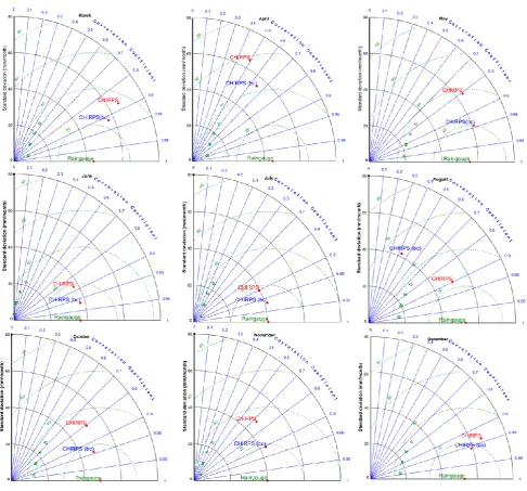
therefore excluded in the analysis. Figure 2 shows the Taylor diagrams displaying the error metrics
264
before and after bias corrections during the wet months of March to May, June-August and October
265
to December with respect to rain gauge data over East Africa. It is illustrated in this figure that
266
Bayesian approach significantly improved the accuracy of the CHIRPS estimates. This is indicated
267
by reduced RMSD and increased correlations for all the months except the month of August. The
268
overcorrection in this month was attributed to erroneous inconsistencies caused by
269
misrepresentation of the rainfall regime by rain gauge data (more details later). The reduction of
270
systematic errors showed dependence on rainfall amounts and were, therefore, more during the
271
months of increased rainfall of April, May and November. This is in line with what was recently
272
documented in (Kimani et al., 2017), that satellite rainfall products underestimate high rainfall
273
amounts over the region.
275
Figure 2: Monthly Taylor diagrams displaying statistical comparison between uncorrected (red) and
276
corrected (blue) CHIRPS estimates with corresponding rain gauge data as the reference. Only the
277
wet months of the rainfall season (March-May and June-August, October-December) over a period
278
of 11 years (2003–2013) were utilized. The azimuthal angle represents correlation coefficient; radial
279
distance the standard deviation (mm/month) and green contours represent RMSD (mm/month).
280
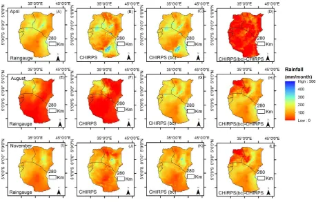
Figure 3 shows the spatial distribution of monthly averaged satellite rainfall estimates before and
281
after bias corrections represented for each season and corresponding rain gauge data. The spatial
282
patterns of bias-corrected (bc) display areas of improved rainfall estimates, and the change maps
283
indicate the areas where correction of CHIRPS estimates was done.
284
It can be observed from rain gauge data high rainfall is over Mt Kenya, Lake Victoria and around
285
Mt Elgon. CHIRPS estimates are able to capture those areas of highest rainfall but show
286
overestimates over southern Tanzania. This overestimation is associated with the consistent high
287
variance of the rain gauge, hence the corrected estimates approach the uncorrected ones. These
288
findings are in line with (Tian et al., 2010) that used the probability distribution to adjust satellite
289
rainfall estimates and associated with corrections to misrepresentation of rainfall variability by the
290
rain gauge network. During JJA seasons represented by August month, the CHIRPS (bc) estimates
291
overestimate rainfall amounts, especially over Mt Kenyan highlands. This again is attributed to
temporal inconsistencies of the patterns in rain gauge spatial rainfall that resulted in overcorrection.
293
However, in November of OND season, the CHIRPS (bc) estimates are close to the rain gauge
294
rainfall and (Kimani et al., 2017) reported CHIRPS underestimations on high elevated areas (over
295
the same study areas) and it is credible that this approach adequately reduced these errors.
296
297
Figure 3: Monthly rainfall averages (2003-2013) of rain gauge data and satellite rainfall estimates
298
before (CHIRPS), after bias corrections (CHIRPS (bc)) and the difference between CHIRPS (bc) and
299
CHIRPS.
300
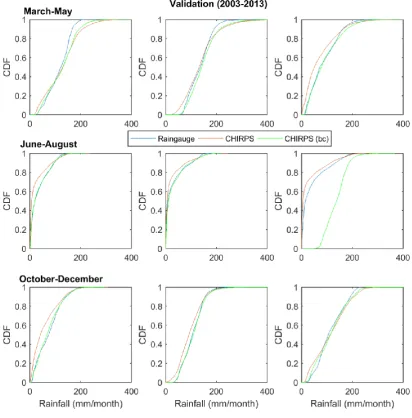
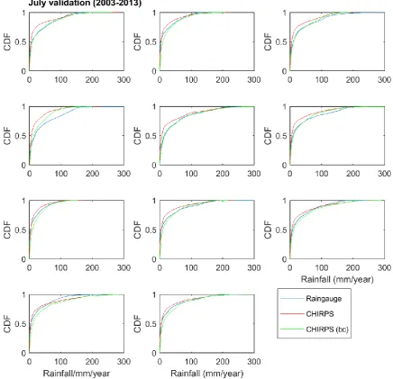
Figure 4 shows the CHIRPS systematic errors adjusted using empirical Cumulative Distribution
301
Function (CDF) plots before and after bias corrections during MAM, JJA and OND rainfall seasons.
302
Before corrections, CHIRPS overestimated the relatively low (<200 mm/month) rainfall amounts
303
and underestimated high (>200 mm/month) amounts. This concurs with (Paredes-Trejo et al., 2017)
304
that CHIRPS monthly estimates overestimate/underestimate low/high rainfall amounts. After bias
305
correction, CHIRPS estimates in each of the nine months show significant change in spatial
306
distribution close to the rain gauge data except in the month of August that show overcorrections.
307
309
Figure 4: Empirical Cumulative Distribution Function (CDF) of monthly rain gauge data, raw
310
satellite rainfall estimates (CHIRPS), and bias-corrected (CHIRPS (bc)) over the validation period
311
(2003–2013).
312
Table 1 shows the monthly error statistics for all the wet months before and after bias corrections.
313
The change of errors for each month is given in percentages. It is evident the bias corrected CHIRPS
314
estimates show reductions in RMSD and MAE errors and increase of correlations. The overall
315
monthly average reduction of RMSD (29-56) % and MAE (28-60) % and correlations increase (2-32)
316
% is an indication of the high skill of the bias correction approach. It can be observed that the bias
317
correction was successful for both high and low rainfall amounts. This is an indication that the
318
dependence of corrected systematic errors not only on overall rainfall magnitudes but also on its
319
distribution and regimes.
320
The corrected errors also showed dependence on seasons and this was indicated by RMSD and
321
MAE reduction patterns that are high during JJA rainfall season. Consequently, a reduction of 50%
322
and 60% of RMSD and MAE respectively were observed in the month of June. These changes are
323
attributed to the onset of south-east monsoon in May that ends by November. This shows the
324
corrected CHIRPS errors follow the rainfall systems affecting rainfall variabilities over East Africa.
325
Table1: Statistics for the monthly spatial evaluation
327
Months RMSD RMSD
(bc)
Change
(%)
MAE MAE
(bc)
Change
(%)
CC CC
(bc)
Change
(%)
Rainfall
(mm)
March 34.9 24.0 -31 24 16 -32 0.87 0.92 5 116
April 57.7 25.6 -56 38 24 -37 0.49 0.65 32 135
May 38.0 20.3 -47 29 14 -51 0.81 0.94 17 86
June 18.7 9.4 -50 14 6 -60 0.87 0.97 11 36
July 17.8 10.4 -42 11 6 -44 0.90 0.97 7 30
August 23.5 51.3 118 15 97 545 0.90 0.43 -52 42
October 31.0 16.1 -48 24 11 -53 0.81 0.94 17 75
November 32.7 18.4 -44 24 13 -45 0.73 0.91 25 106
December 24.5 17.4 -29 18 13 -28 0.94 0.96 2 114
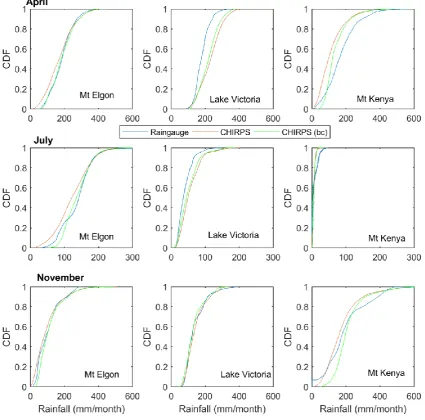
Performances of CHIRPS and CHIRPS (bc) with respect to rain gauge data were further compared
328
over Lake Victoria, Mt Elgon and Mt Kenya during the wettest (April and November) of MAM,
329
OND and driest (JJA) rainfall seasons. These areas are significant in that they experience rainfall of
330
different regimes from local effects. Figure 5 shows the CDFs of the rain gauge data, CHIRPS and
331
CHIRPS (bc) over those areas. It is evident the CDFs of CHIRPS (bc) is aligned closer to those of the
332
rain gauge data in all the months. However, it is also evident in highly elevated areas of Mt Kenya
333
the cumulative distributions of the rain gauge data and CHIRP (bc) were not well aligned. This was
334
more evident during April and November. It is worth noting these two seasons are influenced by
335
ITZC and this large-scale circulation was associated with observed fluctuations in rainfall. These
336
results concur with Sun et al., (2015) study that used model simulation to study the relationship
337
between rainfall over Lake Victoria and surface temperature that showed the relationship is
338
associated to influences of large-scale circulations and orography to rainfall variability. This
339
suggests the systematic errors in the uncorrected CHIRPS may be linked to these external factors.
341
Figure 5: Empirical Cumulative Distribution Function (CDF) of monthly rain gauge data, satellite
342
rainfall estimates (CHIRPS), and bias-corrected CHIRPS (bc) over the validation period (2003–2013).
343
Shown are only areas within which high rainfall amounts are experienced during March-May (Lake
344
Victoria), June-August (Mt Elgon) and October-December (Mt Kenya) as represented by the months
345
of April, July and November respectively.
346
4.2 Yearly spatial distribution of bias corrected CHIRPS
347
In this section yearly CHIRPS and the CHIRPS (bc), estimates are described in cumulative
348
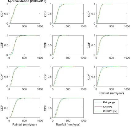
distribution plots in Figures 6, 7, and 8 of the month of April, July and November respectively.
349
In April (Figure 6), it is evident before bias corrections CHIRPS underestimates/overestimates
350
low/high rainfall amounts. Underestimation was more evident in years 2004, 2006 and 2013, which
351
are the wettest years during MAM season and were adjusted to align with rain gauge data. In July
352
(Figure 7), rainfall amount is generally low and general overestimation before correction is
353
observed. The bias correction significantly adjusted the rainfall distribution to match the rain gauge
354
data. However in years 2004, and 2009-2013 the distribution plots show low skills in adjusting the
355
rainfall estimates. From the rainfall averages, 2004 and 2009 are years with anomalous wet rain
356
gauge records which explains the source of over-corrections.
Similar overcorrection is evident in Figure 8 in 2013 and this one of the driest year during the
358
validation period in OND rainfall season. From these results, it is clear that during MAM more
359
systematic errors were reduced that corresponds to years of high rainfall amounts. However,
360
during JJA and OND changes in the frequency of extreme rainfall amounts relative to other years
361
caused irregularities of errors and over corrections resulted. The seasonality of the anomalous years
362
suggests external influences.
363
364
Figure 6: Empirical Distribution Function (CDF) of rain gauge data raw satellite rainfall estimates
365
(CHIRPS), bias-corrected CHIRPS (bc) over the validation period (2003–2013) of the month of April.
367
Figure 7: The same as Figure 6, except for the month of July.
368
370
Figure 8: The same as Figure 6, except for the month of November.
371
The statistics of yearly evaluation are summarized in Table 2. The improvement in spatial pattern
372
during the three rainfall seasons as represented by each month show reduced RMSD (mm/year)
373
and MAE (mm/year), and the corresponding increase in correlations. It is evident, in April the
374
corrected large systematic errors correspond with years of high rainfall and consequently, the dry
375
years have fewer errors. The wettest year (2006) show the highest change in correlations (77%) and
376
the driest year (2009) the least (<10%). In July, there is a significant reduction of errors but the
377
approach showed low skills in eradicating errors of anomalous increased rainfall observed in the
378
years 2004 and 2009. About four times rainfall magnitudes different from other validation years
379
was observed during these two years leading to inconsistent errors. Similar to July, in November,
380
significant errors were reduced but in the anomalous dry year in 2013, least errors were corrected
381
and overcorrection was observed. RMSD and MAE increased, while correlations decreased
382
meaning besides errors dependence on rainfall magnitudes the consistencies of the errors
inter-383
annually affect the performance. The randomness of the errors is evident in the inter-annual
384
analysis.
385
386
388
Table2: Statistics for the yearly spatial evaluation
389
April RMSD RMSD
(bc)
Change
(%)
MAE MAE
(bc)
Change
(%)
CC CC
(bc)
Change Rainfall
2003 66.7 55.1 -17 49 40 -19 0.56 0.70 24 134
2004 79.7 68.3 -14 56 44 -21 0.39 0.48 24 158
2005 50.8 40.5 -20 37 28 -23 0.57 0.68 20 109
2006 109.4 98.1 -10 77 68 -11 0.09 0.15 77 179
2007 51.5 40.9 -21 39 29 -25 0.63 0.74 18 117
2008 64.9 54.4 -16 45 36 -21 0.60 0.67 12 123
2009 61.6 56.2 -9 42 39 -7 0.61 0.66 8 116
2010 65.5 50.2 -23 47 35 -27 0.61 0.73 19 135
2011 80.3 73.5 -9 46 39 -13 0.60 0.63 4 103
2012 68.5 59.2 -13 49 41 -16 0.67 0.75 13 152
2013 85.4 74.1 -13 60 51 -15 0.44 0.58 31 161
July RMSD RMSD
(bc)
Change (%)
MAE MAE
(bc)
Change (%)
CC CC
(bc)
change Rainfall
2003 23.8 15.4 -35 14 8 -41 0.85 0.94 10 30
2004 17.1 15.6 -9 9 10 2 0.85 0.90 6 203
2005 26.4 20.0 -24 15 11 -25 0.87 0.92 6 33
2006 38.5 29.2 -24 22 18 -20 0.73 0.85 16 39
2007 26.2 20.1 -23 16 11 -33 0.90 0.94 4 42
2008 32.1 21.6 -33 17 12 -31 0.82 0.92 11 36
2009 14.0 16.3 16 8 10 26 0.84 0.82 -2 164
2010 22.1 14.1 -36 12 9 -25 0.88 0.95 8 28
2011 26.8 22.6 -15 15 12 -19 0.84 0.91 8 30
2012 29.8 30.5 3 14 15 4 0.84 0.88 5 24
2013 22.9 18.5 -19 12 10 -16 0.88 0.92 5 28
November RMSD RMSD
(bc)
Change
(%)
MAE MAE
(bc)
Change
(%)
CC CC
(bc)
change Rainfall
2003 50.6 32.8 -35 32 22 -32 0.67 0.86 28 88
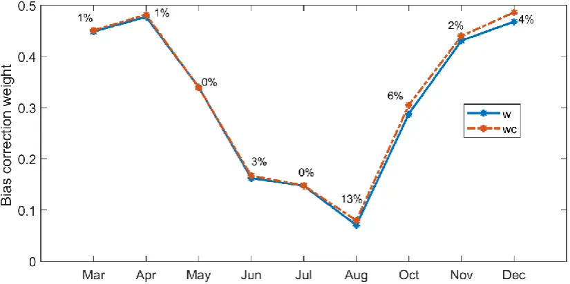
Further analysis was carried out to determine the influence of large-scale circulations to satellite
390
rainfall systematic errors in CHIRPS. This was done by assessing the impact of excluding
391
anomalous wet years (1997/1998) during El Niño. Figure 9 and 10 show the spatial and temporal
392
distribution of bias correction weight when the El Niño years of 1997/1998 are included (w) and
393
excluded (wc) and the difference (wc-w) respectively. From the weight distribution map in figure 9
394
during MAM and JJA rainfall months of April and July respectively, no significant difference occurs
395
in bias correction weight. However, in November, increased performance after correction of
396
systematic errors is evident particularly over Lake Victoria, southwestern Tanzania and Eastern
397
Kenya. These changes are supported by temporal analysis in figure 10 where significant changes
398
are observed from the month of August and including the OND rainfall months. It can be depicted
399
that general circulations related to El Niño are associated with CHIRPS systematic errors observed
400
inter-annually. These findings concur with the study (Indeje et al., 2000) that during this period
401
influences of El Niño–Southern Oscillation (ENSO) are experienced over East Africa. The rainfall
402
variabilities in Lake Victoria are also linked to largescale circulations (Sun et al., 2015). It is therefore
403
evident that the interannual systematic errors of CHIRPS and any other satellite-derived rainfall
404
estimates can be reduced more effectively by a prior knowledge of the external factors influencing
405
the rainfall variabilities.
406
2005 29.2 23.1 -21 21 17 -22 0.72 0.82 14 583
2006 81.9 66.2 -19 62 51 -19 0.67 0.76 12 205
2007 34.6 27.9 -19 26 21 -19 0.77 0.85 10 79
2008 50.4 36.1 -28 36 27 -25 0.38 0.62 65 108
2009 36.5 32.5 -11 28 25 -9 0.76 0.79 3 97
2010 30.5 24.3 -20 21 18 -16 0.78 0.88 13 66
2011 75.4 59.1 -22 51 43 -17 0.63 0.75 20 176
2012 45.1 43.7 -3 33 30 -9 0.62 0.64 4 97
407
Figure 9: Spatial distributions of raingauge correction weights before (w) and after (wc) exclusion of
408
El Niño years (1997/1998) during training in the three rainfall season months of April, July and
409
November. The weights are derived from the variances of the rain gauge data and those of the
410
corresponding satellite rainfall estimates. Mean (1981-2013) wind patterns are embedded on the
411
maps and the arrows point in the direction of wind flow and the size of the arrow represents the
412
wind speed.
413
414
Figure 10: Temporal changes of bias correction weights before (w) and after (w c) exclusion of El
415
Niño years (1997/1998) during training in the three rainfall season months of April, July and
416
November. The weights are derived from the variances of the rain gauge data and those of the
417
corresponding satellite rainfall estimates.
5. Conclusions
419
Rain gauge distributions are on the decline and satellite rainfall estimates are increasingly used to
420
complement the sparse rain gauge data. However, rain gauge data is used as reference data to
421
validate the incoming satellite products but with the decreasing trend, the quality of this validation
422
may be compromised. To solve this problem Bayesian approach is hereby applied to the existing
423
historical rain gauge information to create a consistent satellite rainfall data that can be used for
424
climate studies. A long term temporal scale (monthly) bias correction is therefore applied on
425
Climate Hazards Group Infrared Precipitation with Stations (CHIRPS v2) data to reduce systematic
426
errors using a corresponding gridded (0.05o) rain gauge data over East Africa. The gridded rain
427
gauge data was developed by ICPAC intergovernmental organization to safeguard the decreasing
428
network. The choice of CHIRPS was based on its close correspondence with rain gauge data over
429
the region [6] and its period of long coverage suitable for climate studies. Satellite rainfall products
430
exhibit systematic errors and although CHIRPS show good performance over East Africa, reducing
431
these errors would increase its performances for climate studies, and agricultural and water
432
management. The study aimed at temporally and spatially evaluating how CHIRPS rainfall
433
estimates compare with the gridded rain gauge data in magnitude and distributions after bias
434
correction. Only the wet rainfall months of MAM, JJA and OND are utilized for a period of 33 years
435
of which 22 years were for calibration and 11 years for validation.
436
Monthly analysis showed CHIRPS estimates have systematic errors mainly of underestimations
437
and application of the Bayesian method adequately reduced such errors. The remaining errors after
438
correction showed dependence on rainfall magnitudes and hence increased with increase in rainfall
439
amounts. The highest change in correlation coefficients of 32% in April, and 25% in November
440
which are the peak rainfall months of MAM and OND rainfall seasons were observed. Cumulative
441
distributions plots revealed that in areas of low rainfall (<200mm/month) the corrected errors were
442
associated with overcorrections beyond which underestimations were dominant. Remarkably the
443
approach significantly reduced these errors except in August when the presence of a different
444
rainfall regime produced irregular errors in rain gauge data that were observed as overcorrections.
445
The corrected CHIRPS estimates showed dependence on seasons and this was indicated by patterns
446
of reduction in RMSD and MAE that were highest during JJA rainfall season. Consequently, a
447
reduction of RMSD (50%), and MAE (60%) were observed in the month of June. These changes
448
coincide with the onset of south-east monsoon that peak in the month of May of MAM season and
449
includes JJA rainfall season. This shows the bias corrected CHIRPS follow the rainfall systems
450
affecting rainfall variabilities over East Africa. The overall monthly RMSD and MAE are reduced
451
between (26-48) % and (28-60) % respectively and correlations increase between 2-32 %. It can be
452
concluded that the Bayesian approach reduced CHIRPS errors of monthly scale which were locally
453
induced, like topographic and lake processes.
454
The areas of highest systematic error reductions include the high elevated areas especially Mt
455
Kenya, Mt Elgon and Lake Victoria region. These areas are also significant because of the mixed
456
rainfall regimes influenced by local effects. Performances of CHIRPS and CHIRPS (bc) with respect
457
to rain gauge data were further compared over these areas (Figure1) during the wettest (April and
458
November) and driest (July) months of MAM, OND and JJA rainfall seasons respectively. The
459
results showed that even though the areas differ in the amount of rainfall in each season, the bias
460
correction aligned the CHIRPS cumulative distribution closer to that of the rain gauge data.
461
However, on highly elevated areas of Mt Kenya, the cumulative distributions of the rain gauge data
462
and CHIRP (bc) were not well aligned. This was more evident during April and November, of
463
MAM and OND rainfall seasons and this was associated with largescale influences as the two
464
seasons are experienced during ITCZ overpass.
Interannual CHIRPS bias correction assessments were carried out with respect to rain gauge data
466
for the months of April, July and November to represent MAM, JJA and OND rainfall seasons.
467
Spatial rainfall patterns revealed that systematic errors exist in yearly estimates mainly of
468
underestimation which increased with increase in rainfall magnitudes. However cumulative
469
distribution analysis showed CHIRPS estimates bias correction adjusted
470
underestimations/overestimations of low/high rainfall amounts. Underestimation was more during
471
extreme wet years (2004, 2006 and 2011), which were shown in error statistics with highest rainfall
472
amounts. However, the bias correction adjusted the CHIRPS estimates to align with rain gauge
473
data. Similar to monthly analysis, MAM interannual systematic errors were mainly related to
474
rainfall magnitudes and rainfall distributions and were effectively reduced.
475
During JJA and OND rainfall seasons CHIRPS systematic errors associated with rainfall magnitude
476
and distribution were reduced. However, over corrections were observed in extreme wet and dry
477
years which were attributed to irregularities of rainfall patterns that were not well captured by the
478
rain gauge data. The overall monthly statistics measures a reduction of RMSD (29-56) % and MAE
479
(28-60) % and an increase of correlations (2-32) %. For yearly analysis they are reductions of RMSD
480
(9-23) %, and MAE (7-27) % and increase of correlations (4-77) % for MAM months, reduction of
481
RMSD (15-35) % and MAE (16-41) % and increase in correlations (5-16)% for JJA months, and
482
reduction of RMSD (3-35) % and MAE (9-32) % and increase of correlations (3-65)% for OND
483
months.
484
The impacts of largescale phenomena on systematic errors in CHIRPS were assessed by exclusion of
485
known anomalous wet years (El Niño) of 1997/1998 over East Africa. The result showed a
486
significant spatial reduction of these errors more evident from the month of August (13%) and
487
OND (between 2-6%) rainfall months. Minimal (1%) impacts were observed during MAM rainfall
488
months and were observed mainly in areas around Lake Victoria, Eastern Kenya and southwest
489
Tanzania. These are areas associated with large-scale circulation of ENSO (Lake Victoria) and
low-490
level Turkana jet (Eastern Kenya). In conclusion, the bias corrected CHIRPS estimates are more
491
representative of the rainfall magnitude and distribution. Further, these data and the associated
492
errors are more informative of local and large-scale influences over East Africa and can, therefore,
493
be used for climate studies. The approach is recommended for other areas and to other products.
494
However, prior long-term analysis is advised to exclude anomalous years and correct them
495
separately. The approach is suitable for long-term data correction where consistencies of errors can
496
be assumed.
497
Supplementary Materials: Bayesian Bias Corrected Rainfall generated data in this study.
498
Acknowledgments: This work was made possible through the funding provided by the Netherlands Fellowship
499
Programmes (NFP), and we greatly appreciate their support. The University provided funds for open access.
500
Author Contributions: All three authors contributed in concept building and manuscript preparation.
501
Kimani analyzed the data and drafted the manuscript. Su and Hoedjes provided conceptual advice and
502
contributed to the overall writing and approval of the final manuscript.
503
Conflict of Interest: The authors declare no conflict of interest.
504
References
505
506
1. Kidd, C.; Bauer, P.; Turk, J.; Huffman, G.J.; Joyce, R.; Hsu, K.L.; Braithwaite, D.
507
Intercomparison of high-resolution precipitation products over northwest europe. J.
508
Hydrometeorol. 2012, 13, 67-83.
2. Sorooshian, S.; Hsu, K.L.; Gao, X.; Gupta, H.V.; Imam, B.; Braithwaite, D. Evaluation of
510
persiann system satellite-based estimates of tropical rainfall. Bull. Amer. Meteorol. Soc. 2000,
511
81, 2035-2046.
512
3. Feidas, H.; Lagouvardos, K.; Kotroni, V.; Cartalis, C. Application of three satellite techniques
513
in support of precipitation forecasts of a nwp model. Int J Remote Sens 2005, 26, 5393-5417.
514
4. Maidment, R.I.; Grimes, D.I.F.; Allan, R.P.; Greatrex, H.; Rojas, O.; Leo, O. Evaluation of
515
satellite-based and model re-analysis rainfall estimates for uganda. Meteorological Applications
516
2013, 20, 308-317.
517
5. Tote, C.; Patricio, D.; Boogaard, H.; van der Wijngaart, R.; Tarnavsky, E.; Funk, C. Evaluation
518
of satellite rainfall estimates for drought and flood monitoring in mozambique. Remote
519
Sensing 2015, 7, 1758-1776.
520
6. Kimani, M.W.; Hoedjes, J.C.B.; Su, Z.B. An assessment of satellite-derived rainfall products
521
relative to ground observations over east africa. Remote Sensing 2017, 9.
522
7. Abera, W.; Brocca, L.; Rigon, R. Comparative evaluation of different satellite rainfall
523
estimation products and bias correction in the upper blue nile (ubn) basin. Atmospheric
524
Research 2016, 178, 471-483.
525
8. AghaKouchak, A.; Mehran, A.; Norouzi, H.; Behrangi, A. Systematic and random error
526
components in satellite precipitation data sets. Geophysical Research Letters 2012, 39.
527
9. Mateus, P.; Borma, L.S.; da Silva, R.D.; Nico, G.; Catalao, J. Assessment of two techniques to
528
merge ground-based and trmm rainfall measurements: A case study about brazilian amazon
529
rainforest. Giscience & Remote Sensing 2016, 53, 689-706.
530
10. Maurer, E.P.; Pierce, D.W. Bias correction can modify climate model simulated precipitation
531
changes without adverse effect on the ensemble mean. Hydrology and Earth System Sciences
532
2014, 18, 915-925.
533
11. Cressman, G.P. An operational objective analysis system. Mon.Weather Rev 1959, 367 – 374.
534
12. Vila, D.A.; de Goncalves, L.G.G.; Toll, D.L.; Rozante, J.R. Statistical evaluation of combined
535
daily gauge observations and rainfall satellite estimates over continental south america. J.
536
Hydrometeorol. 2009, 10, 533-543.
537
13. Tian, Y.D.; Peters-Lidard, C.D.; Eylander, J.B. Real-time bias reduction for satellite-based
538
precipitation estimates. J. Hydrometeorol. 2010, 11, 1275-1285.
539
14. Stokstad, E. Hydrology - scarcity of rain, stream gauges threatens forecasts. Science 1999, 285,
540
1199-1200.
541
15. Funk, C.; Hoell, A.; Shukla, S.; Blade, I.; Liebmann, B.; Roberts, J.B.; Robertson, F.R.; Husak,
542
G. Predicting east african spring droughts using pacific and indian ocean sea surface
543
temperature indices. Hydrology and Earth System Sciences 2014, 18, 4965-4978.
544
16. Funk, C.C.; Peterson, P.J.; Landsfeld, M.F.; Pedreros, D.H.; Verdin, J.P.; Rowland, J.D.;
545
Romero, B.E.; Husak, G.J.; Michaelsen, J.C.; Verdin, A.P. A quasi-global precipitation time
546
series for drought monitoring: U.S. Geological survey data series 832, 4 p. 2014.
547
17. Suwendi, A.; Allebach, J.P. Nearest-neighbor and bilinear resampling factor estimation to
548
detect blockiness or blurriness of an image. Journal of Electronic Imaging 2008, 17.
549
18. Carlin, B.P.; Louis, T.A. Bayes and empirical bayes methods for data analysis, chapman and
550
hall, london, uk. 1996; p 399 pp.
19. Talagrand, O. Assimilation of observations, an introduction (gtspecial issueltdata
552
assimilation in meteology and oceanography: Theory and practice). Journal of the
553
Meteorological Society of Japan. Ser. II 1997, 75, 191-209.
554
20. Taylor, K.E. Summarizing multiple aspects of model performance in a single diagram. Journal
555
of Geophysical Research-Atmospheres 2001, 106, 7183-7192.