https://doi.org/10.5194/amt-11-5981-2018 © Author(s) 2018. This work is distributed under the Creative Commons Attribution 4.0 License.
Recovery of the three-dimensional wind and sonic temperature data
from a physically deformed sonic anemometer
Xinhua Zhou1,2,3, Qinghua Yang1, Xiaojie Zhen4, Yubin Li5, Guanghua Hao6, Hui Shen6, Tian Gao2, Yirong Sun2, and Ning Zheng3
1Guangdong Province Key Laboratory for Climate Change and Natural Disaster Studies, School of Atmospheric Sciences, Sun Yat-sen University, Zhuhai 519082, China
2CAS-CSI Joint Laboratory of Research and Development for Monitoring Forest Fluxes of Trace Gases and Isotope Elements, Institute of Applied Ecology, Chinese Academy of Sciences, Shenyang 110016, China
3Campbell Scientific Incorporation, Logan, Utah 84321, USA 4Beijing Techno Solutions Ltd., Beijing 100089, China
5Nanjing University of Information Science and Technology, Nanjing 210044, China 6National Marine Environmental Forecasting Center, Beijing 100081, China
Correspondence:Qinghua Yang ([email protected]) and Ning Zheng ([email protected]) Received: 26 March 2018 – Discussion started: 22 June 2018
Revised: 23 September 2018 – Accepted: 2 October 2018 – Published: 30 October 2018
Abstract.A sonic anemometer reports three-dimensional (3-D) wind and sonic temperature (Ts)by measuring the time of ultrasonic signals transmitting along each of its three sonic paths, whose geometry of lengths and angles in the anemometer coordinate system was precisely determined through production calibrations and the geometry data were embedded into the sonic anemometer operating system (OS) for internal computations. If this geometry is deformed, al-though correctly measuring the time, the sonic anemome-ter continues to use its embedded geometry data for inanemome-ternal computations, resulting in incorrect output of 3-D wind and
Tsdata. However, if the geometry is remeasured (i.e., recal-ibrated) and to update the OS, the sonic anemometer can re-sume outputting correct data. In some cases, where immedi-ate recalibration is not possible, a deformed sonic anemome-ter can be used because the ultrasonic signal-transmitting time is still correctly measured and the correct time can be used to recover the data through post processing. For ex-ample, in 2015, a sonic anemometer was geometrically formed during transportation to Antarctica. Immediate de-ployment was critical, so the deformed sonic anemometer was used until a replacement arrived in 2016. Equations and algorithms were developed and implemented into the post-processing software to recover wind data with and without transducer-shadow correction and Ts data with crosswind
correction. Post-processing used two geometric datasets, pro-duction calibration and recalibration, to recover the wind and
Ts data from May 2015 to January 2016. The recovery re-duced the difference of 9.60 to 8.93◦C between measured and calculatedTs to 0.81 to−0.45◦C, which is within the expected range, due to normal measurement errors. The re-covered data were further processed to derive fluxes. As data reacquisition is time-consuming and expensive, this data-recovery approach is a cost-effective and time-saving option for similar cases. The equation development can be a refer-ence for related topics.
1 Introduction
5982 X. Zhou et al.: Recovery of the three-dimensional wind and sonic temperature data
sonic temperature and, when combined with fast-response scalar sensors, the fluxes of CO2, H2O, and other atmo-spheric constituents.
It has three pairs of sonic transducers forming three sonic paths (Fig. 1), each of which is between paired sonic trans-ducers. The three paths are situated as optimized angles for wind measurements in the 3-D anemometer coordinate sys-tem, structuring the geometry of sonic anemometer. This ge-ometry is quantitatively defined by the path lengths and path angles that are precisely measured during production cali-bration. A sonic anemometer measures the time of ultrasonic signals transmitting along each path (hereafter, referred as transmitting time). In reference to the sonic path length, the transmitting time is used to calculate the speeds of flow and sound along the path, which will be detailed in Sect. 4 as fol-lows. According to the angles of three sonic paths, the speeds from the three paths are expressed in the 3-D anemometer coordinate system for wind and as sonic temperature for air heat property.
A sonic anemometer has geometry information embed-ded into its operating system (OS) for internal data pro-cessing (see Appendix A), allowing output of 3-D wind and sonic temperature. However, if it is geometrically deformed from the manufacturer’s setting at millimeter scales, or even smaller, due to an unexpected physical impact in transporta-tion, installatransporta-tion, or other handling, the geometry embed-ded in the OS is not representative of the current geometry of this sonic anemometer. As a result, the anemometer no longer outputs correct wind speeds and sonic temperatures because the deformation in geometry changes the relative spatial relationship among its six sonic transducers. If, an impact displaces a transducer relative to the others, the dis-placement must change at least one of the sonic path lengths and one of the sonic path angles. Fortunately, if geometrical deformation is the only problem, rather than physical dam-age to the transducers, the sonic anemometer can, according to its working physics (Schotland, 1955), correctly perform its transmitting-time measurements. Due to the change in a sonic path length, the speeds of air flow and sound along the path are incorrectly computed because the sonic path length embedded in the OS does not match the true length when the transmitting time was measured. As a result, the incorrect speeds along with the change in any sonic path angle might cause all 3-D wind speeds as well as sonic temperature out-puts to be incorrect. These incorrect outout-puts are recoverable because the transmitting time was correctly measured and the deformed geometry can be remeasured (i.e., recalibrated) by the manufacturer to whom the anemometer can be shipped back with care. However, the equations and algorithms for the recovery are needed if a sonic anemometer is found to be geometrically deformed in a remote site where its use has to be continued. From such a site, it could take months, seasons, or even longer for a deformed anemometer to be transported back to the manufacturer for geometry remeasurements, re-calibration, and shipped back to the site. In this case, if the
measurements were not continued, a measurement season or year could be easily missed.
This study demonstrates data recovery from such a case when a sonic anemometer as a component of the IRGA-SON (integrated CO2/H2O open-path gas analyzer and 3-D sonic anemometer, Campbell Scientific Inc., 2018) was ge-ometrically deformed during transportation to the Antarc-tic Zhongshan Station from China in early 2015 and had to be used until its replacement arrived at the site early the next year. If the deformed sonic anemometer was not used, one measurement-year would have been missed because the only transportation of R/V Xue Long (i.e., Snow Dragon in English) from China to the Zhongshan Station served a round-trip to the site on an annual basis. More impor-tantly, the 2015 data were also needed by related projects for collaborations. Therefore, the geometrically deformed sonic anemometer was used to acquire the 2015 data. In early 2016, the deformed anemometer was shipped, with a pair of buffer bumpers for protection, to the manufacturer of Campbell Sci-entific Inc. in the US for remeasurements of its geometry to update its OS (i.e., recalibration).
Using the measurements of sonic path lengths and sonic path angles for this sonic anemometer from production cali-bration in April 2014 before its transportation and from recal-ibration in March 2016 after the field use in the Zhongshan Station, this study aims to develop and verify the equations and algorithms to recover the 2015 data measured using this geometrically deformed sonic anemometer to data as if mea-sured with the this anemometer after recalibration although actually measured before the recalibration, providing a refer-ence to similar cases and/or related topics.
2 Site, instrumentation, and data
The observation site was in the coastal landfast sea ice area of the Zhongshan Station (69◦220S and 76◦220E), East Antarc-tica (Yang et al., 2016; Yu et al., 2017; Zhao et al., 2017). In this area, as influenced by the unique solar cycles, the climate is characterized by the polar night from late March to mid-July and the polar day from mid-November to January. The polar day and the polar night are inhabitable to human life, but drive atmospheric dynamics in a way that is of interest to human beings (Valkonen et al., 2008); therefore, this region has attracted scientists to measure its surface heat balance; However, these measurements are not an easy task in terms of financial support, technical infrastructure, and administra-tive management. As such, only a few studies on such mea-surements have been conducted in this region (e.g., Vihma et al., 2009; Liu et al., 2017).
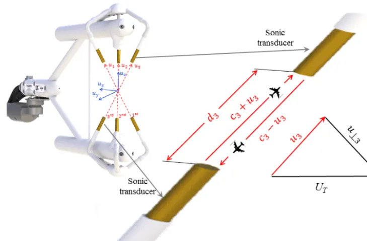
Figure 1.Diagram of the IRGASON for the three sonic measurement paths (red dash lines) along which ultrasonic signals transmit, and the three dimensional (3-D) right-handed orthogonal anemometer coordinate system (blue lines) in which 3-D wind is expressed (i.e.,u1,u2,
andu3are the flow speeds along the first, second, and third sonic paths, respectively. These three flow speeds are expressed asux,uy, and uzin this 3-D anemometer coordinate system).d3is the third sonic path length,c3is the measured speed of sound along the third sonic path,
andUTis the total flow vector whose magnitude is equal to q
u23+u2⊥3or
q
u2x+u2y+u2z.
flux stations in May 2015. One station (see Fig. 2) was configured with the IRGASON (SN: 1131) for the fluxes, four-component net radiometer (model: CNR4, Kipp & Zo-nen, Delft, the Netherlands) for net radiation and radia-tion fluxes; one temperature and relative humidity probe (model: HMP155A, SN: H5140031, Vaisala, Helsinki, Fin-land) inside a 14-plate naturally aspirated radiation shield of model 41005 for air temperature and air relative humid-ity; and one infrared radiometer (model: SI-111, SN: 2962, Apogee, UT, USA) for surface temperature. In early 2016, a CSAT3B (Campbell Scientific Inc., UT, USA) was added for additional data of 3-D wind and sonic temperature. This OPEC station was also equipped with a built-in barome-ter (model: MPXAZ6115A, Freescale Semiconductor, TX, USA) for atmospheric pressure and a built-in 107 temper-ature probe (model: 100K6A1A, BetaTherm, Finland) in-side a 6-plate naturally aspirated radiation shield of model 41303-5A for air temperature, the IRGASON was connected to and controlled by an EC100 electronic module (SN: 1542, OS: EC100.04.10) that, in turn, was connected to and in-structed by a central CR3000 Measurement and Control Datalogger (SN: 7720, OS 25) for these sensor measure-ments, data processing, and data output. While receiving the data output from EC100 at 10 Hz, the CR3000 also con-trolled and measured slow response sensors at 0.1 Hz such as the CNR4, HMP155A, and others in support to this study.
EasyFlux_CR3OP (version 1.00, Campbell Scientific Inc., 2016) was used inside CR3000. The data of 3-D wind, sonic temperature, CO2and H2O amounts, atmospheric pressure, diagnosis codes for the 3-D sonic anemometer and open-path infrared gas analyzer, air temperature, and relative humidity were stored 10 records per second (i.e., 10 Hz). The data from all sensors were computed and stored by the CR3000 at every half-hour interval.
3 Data check and instrument diagnosis
Immediately after the station started to run, all measured values were checked. Unfortunately, the sonic temperature from the 3-D sonic anemometer was incorrect because it was around 10◦C higher than the air temperature from HMP155A or 100K6A1A. Given a H2O density of about 1.00 g m−3and air temperature about−20◦C, sonic
temper-ature should be around 0.13◦C higher than air temperature
5984 X. Zhou et al.: Recovery of the three-dimensional wind and sonic temperature data
Figure 2. The eddy-covariance station located in the coastal landfast sea ice area of Antarctica Zhongshan Station (69◦220S, 76◦220E). It was configured with the IRGASON integrated CO2/H2O open-path gas analyzer and three-dimensional sonic anemometer, CNR4 four-component net radiometer, HMP155A air temperature and relative humidity probe, and SI-111 infrared ra-diometer.
while the station was running. Apparently, the largest abso-lute difference in sonic temperature among the three paths reached 17◦C, although the difference from an IRGASON sonic anemometer was expected to be < 1◦C. Such a large unexpected absolute difference (e.g., 17◦C) among the three values from the three sonic paths might be caused by the geometrical deformation of sonic anemometer. To confirm the diagnosis, the body of the IRGASON was visually ex-amined and painting on the knuckle of side one (i.e., first sonic path) among the top three claws was found removed as it was apparently impacted (Fig. 3). Therefore, with confi-dence, it was concluded that the incorrect outputs of sonic temperature were caused by the geometrical deformation of sonic anemometer while being transported to Antarctica from China. The deformation also might cause the incorrect outputs of 3-D wind. Therefore, this IRGASON should have been shipped back to the manufacturer for remeasurements of its geometry to update its OS (recalibration). However, as addressed in the introduction, the 2015 data would have been missed if it was shipped back to the manufacturer at that point. To make measurements as planned, this IRGA-SON continued its field duty until the next round-trip of R/V
Xue Long to Antarctica from China until the end of 2015 when its replacement from the manufacturer arrived at the site.
In early 2016, it was replaced in the field and was shipped back to the manufacturer, where it was remeasured for sonic geometry in the recalibration process in March. The remea-surements verified our diagnosis conclusion that the IRGA-SON sonic anemometer was geometrically deformed (see Ta-ble A1 in Appendix A). Therefore, the 2015 data from this sonic anemometer needed to be recovered as if measured by
Figure 3.Painting removed where it was apparently impacted on the knuckle of side claw (first sonic path) among the top three sonic transducer claws of the IRGASON sonic anemometer (serial no.: 1131).
the same anemometer after recalibration, although the data were acquired from the measurements before the recalibra-tion.
4 Algorithm to recover the data of 3-D wind and sonic temperature
An IRGASON sonic anemometer measures wind flows along its three non-orthogonal sonic paths (i.e., the three sonic paths non-orthogonally situated in relation to each other, see Fig. 1), each of which is between a pair of sonic transduc-ers. Sensing each other in each sonic path, the pair separately pulse two ultrasonic signals in opposite directions at the same time. The signal pulsed by the transducer facing the air flow direction along the sonic path takes less time to be sensed by its paired one than the one pulsed by the transducer against the air flow direction. In a path, the transmitting time of the ultrasonic signal upward [tuiwhere subscriptican be 1, 2, or 3, denoting the sequential order of sonic path (Fig. 1). This subscript denotes the same variable throughout] and down-ward (tdi)are measured by the sonic anemometer (Hanafusa, 1982; Foken, 2017). In the case shown in Fig. 1 for the third sonic path, ori=3, the transmitting time of ultrasonic signal upward in the path is given by the following equation:
tu3=
d3
c3+u3
, (1)
the following equation:
td3=
d3
c3−u3
. (2)
4.1 Recovery of 3-D wind data
4.1.1 Algorithm of sonic anemometer to output the 3-D wind data
Equations (1) and (2) lead to
u3=
d3 2
1
tu3 − 1
td3
. (3)
Using the same procedure,u1andu2(see Fig. 1) can be de-rived as the same form. In reference to Eq. (3), the equation forui; wherei=1,2, or 3; can be expressed as follows:
ui= di
2
1
tui − 1
tdi
. (4)
Similar to d3,d1 andd2 are also precisely measured using CMM. The three flow speeds of ui (i=1, 2, or 3) from the three non-orthogonal paths are expressed in the 3-D anemometer coordinate system ofx,y, andz; wherexandy
are the horizontal coordinate axes andzis the vertical axis; and through a transform matrix Aas the 3-D wind speeds (ux,uy, anduz)commonly used in practical applications:
ux uy uz
=A
u1 u2 u3
, (5)
where the 3-D anemometer coordinate system (see Figs. 1 and A1) is defined by its origin at the center of sonic mea-surement volume, theux−uy plane, parallel to the imagery plane, leveled by a built-in bubble in the anemometer struc-ture, and theuy−uzplane through the first sonic path andA is a 3×3 matrix constructed using precisely measured geom-etry of the sonic paths in angles relative to the 3-D anemome-ter coordinate system (see its derivations in Appendix A). MatrixAis unique for each sonic anemometer and is embed-ded in its OS; therefore, the 3-D wind data outputted from the anemometer are the three components ofux,uyanduzin the 3-D anemometer coordinate system.
Due to shadowing from the sonic transducer itself (trans-ducer shadowing), the measured ui is assumed to be lower than its true value in magnitude (Wyngaard and Zhang, 1985; Kaimal and Finnigan, 1994). As denoted byuTi_nwhere sub-scriptT indicates “True” and subscriptnindicates thatuTi_n was estimated from n counts of iterations of transducer-shadow correction as shown in Appendix B, this true value is assumed to be approached through the transducer-shadow correction fromui. Now, the shadow correction was imple-mented as an option if the OS of EC100 for the IRGASON
sonic anemometer is version 5 or newer. Therefore, depend-ing on the option, Eq. (5) alternatively can be expressed as follows: ux uy uz
=A
uT1_n uT2_n uT3_n
. (6)
Following Host et al. (2015), based on Wyngaard and Zhang (1985), the correction equation for the sonic trans-ducer size and sonic path geometry of the IRGASON sonic anemometer is given by
uT i_1=
ui 0.84+0.16 sinαi
, (7)
whereαi is the angle of the total wind vector to the wind vector along sonic pathiand is unknown before the two vec-tors are estimated, but, referencing Figs. 1 and 4, the sinαiin Eq. (7) can be alternatively expressed as a function of flow speed values to lead Eq. (7) as follows:
uT i=
ui
0.84+0.16 q
UT2−u2T i UT
, (8)
whereUTis the magnitude of total true wind vector, given by
UT=
q
u2
x+u2y+u2z. (9)
In Eq. (8), all independent variables are actually related to the variables in Eq. (5). As such, using this equation,uT ican be computed; however, there are two inconvenient issues in this equation application to transducer-shadow corrections: (1) an analytical solution foruT iis not easily available becauseuT i is in a second order term under a square root in the right side of Eq. (8), althoughuT i is analytically expressed in its left side and (2)UT is not available either because ux,uy, anduzare derived fromu1,u2, andu3before the transducer-shadow corrections. Fortunately, the corrections are small in magnitude, as shown in Eq. (8); therefore,ui is closed to uT i. As a result, ux, uy, and uz from Eq. (5) are close to those from Eq. (6). Accordingly, an iteration algorithm may be the right approach to the corrections using Eq. (8), or for the estimation ofuT i.
For the first iteration,uT iin the right side of Eq. (8) could be replaced withui as its estimation. Given thatUTshould be calculated usingux,uy, anduz from Eq. (6), before the transducer-shadow corrections, UT can be estimated using
ux,uy, anduzfrom Eq. (5); see Appendix B: Iteration algo-rithm for sonic transducer-shadow corrections. The iterations ensure that the difference inux,uy, or uz between the last and previous iterations are<1 mm s−1≈1.96σ< 1, where
5986 X. Zhou et al.: Recovery of the three-dimensional wind and sonic temperature data
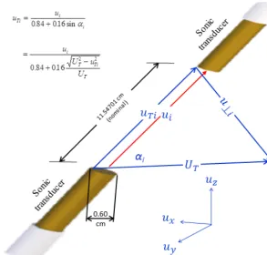
Figure 4. Sonic transducer shadowing along theith (i=1, 2, or 3) sonic path between the two sonic transducers,ui is the measured
magnitude of flow vector whose true magnitude isuT i;u⊥iis the flow speed normal to theith sonic path;ux,uy, anduzare the wind speeds
expressed in the three-dimensional orthogonal anemometer coordinate system; andαi is the angle between sonic pathiand the total flow
vector (UT)equal to q
u2i +u2⊥i or
q
u2x+u2y+u2z. See Wyngaard and Zhang (1985) and Kaimal and Finnigan (1994) for the equation to
calculateuT i.
4.1.2 Procedure to recover 3-D wind data
As addressed in Eqs. (4) to (6), a sonic anemometer mea-sures tui andtdi to calculate the 3-D wind of ux,uy, and uz; therefore, sonic path lengths (di)in Eq. (4) and trans-form matrix A in Eqs. (5) and (6) are embedded into the OS of sonic anemometer in the manufacture processes (see the embedded data for our study sonic anemometer in Ap-pendix A). If the anemometer was physically deformed in transportation, installation, or other handling; the sonic path lengths and sonic path angles must be changed from what they were at the time whendiandAwere embedded into its OS; therefore,diin Eq. (4) and sonic path angles reflected by Ain Eqs. (5) and (6) are no longer valid for this anemome-ter. Consequently; the output ofux,uy, anduzstill based on embeddeddiandAfrom production calibration or recalibra-tion process are erroneous. To correct the erroneous output
ux,uy, anduz need to be transformed back intotui andtdi and be recalculated usingtui andtdi based on the true sonic path lengths and true sonic path angles at the time whentui andtdi were measured in the field by the sonic anemometer physically deformed away from the manufacturer’s geomet-rical settings before its field deployment.
For the true sonic path lengths and true sonic path an-gles, the IRGASON (SN: 1131) was returned to the manu-facturer in the way described in Sect. 3. In the same way as in the manufacture process, the lengths and angles were re-measured using CMM. The rere-measured lengths are denoted bydT i (i=1, 2, or 3) and the remeasured angles were used to reconstruct the transform matrixAasAT(see Appendix A). BothdT i andATare used to update the OS of this IR-GASON for future field uses and to correctux,uy,uz and Ts (sonic temperature, see Sect. 4.2) that were outputted in the field before the remeasurements. The correction proce-dures are different for the output ofux,uy,uzwith or without transducer-shadow corrections.
With transducer-shadow corrections
Transfer ux, uy, and uz in the 3-D anemometer coordi-nate system to the flow speeds along the sonic paths after transducer-shadow corrections.
uT1_n uT2_n uT3_n
=A
−1
ux uy uz
Using Eq. (B5), flow speed along theith sonic path before transducer-shadow correction (ui)can be expressed as fol-lows:
ui=uTi_n
0.84+0.16 q
UT2−u2T i_m
UT
, (11)
where UT can be calculated using Eq. (9) and uT i_m can be reasonably approximated usinguTi_nbecauseuT i_mand uTi_nare close enough to ensureux,uy, anduzto converge at their measurement precision (see Appendix B). Using ui anddi, the time term inside the square bracket in Eq. (4) can be recovered as follows:
1
tui − 1
tdi
=2ui
di
, (12)
Additionally, according to Eq. (4) and usingdT i, the speed of air flow along theith sonic path can be recalculated asuci: uci=
dT i 2
1
tui − 1
tdi
. (13)
Further replacing ui withuci in the iteration algorithm for sonic transducer-shadow corrections in Appendix B, uci is corrected for transducer-shadowing asucT i_n. Using Eq. (6), the recovered vector of 3-D wind in the 3-D anemometer co-ordinate systemucx ucy ucz
0 can be expressed as
fol-lows: ucx ucy ucz
=AT
ucT1_n ucT2_n ucT3_n
. (14)
Without transducer-shadow corrections
Transfer ux,uy, anduz in the 3-D anemometer coordinate system to the flow speeds along individual sonic paths.
u1 u2 u3
=A
−1 ux uy uz (15)
Using Eqs. (12) and (13), the speed of flow along the ith sonic path (uci) is recalculated (i.e., recovered). Based on Eq. (5), the recovered speeds of flow along the three sonic paths can be expressed in the 3-D anemometer coordinate system as follows:
ucx ucy ucz
=AT
uc1
uc2
uc3
. (16)
4.2 Recover sonic temperature data
4.2.1 Algorithm of sonic anemometer to output sonic temperature
Equations (1) and (2) also lead to
c3=
d3 2
1
tu3 + 1
td3
. (17)
Using the same procedure,c1andc2(see Figs. 1 and 5) can be derived as the same form. In reference to Eq. (17), the equation forci, where subscripti=1, 2, or 3; can be ex-pressed as follows:
ci = di
2
1
tui + 1
tdi
(18) Here,ciis the measured speed of sound along the sonic pathi (see Fig. 5). When the crosswind (u⊥i), or wind normal to the sonic pathi, is zero;ci is the true speed of sound (c0i where subscript 0 indicates the speed of sound at crosswind speed equal to zero). Unfortunately, crosswind is rarely zero andci needs to be corrected toc0i. According to Figs. 1 and 5, the true speed of sound is given by
c0i= ci cosαi
= ci
ci/
q
c2i +u2⊥i
=
q
c2i +u2⊥i. (19)
Referencing the diagram for wind vectors in the left side of Fig. 5, this equation can be expressed as follows:
c02i=c2i +UT2−u2T i, (20)
According to the definition of sonic temperature (Kaimal and Finnigan, 1994), the sonic temperature (K) along theith sonic path (Tsi)should be expressed as follows:
Tsi= c20i γdRd
, (21)
whereγd(1.4003) is the ratio of dry-air-specific heat at con-stant pressure (1004 J K−1kg−1)to dry-air-specific heat at constant volume (717 J K−1kg−1)andRdis gas constant for dry air (287.04 J K−1kg−1). The sonic temperature outputted from the sonic anemometer (Tsin◦C) is the average from the three sonic paths (van Dijk, 2002), given by
Ts= 1 3
3
X
i=1
Tsi−273.15= 1 3γdRd
3
X
i=1
c02i−273.15. (22)
Substitutingc0i with Eq. (20) and then substitutingci with Eq. (18),Tscan be expressed as follows:
Ts= 1 3γdRd
( 3
X
i=1
"
di2
4
1
tui + 1
tdi
2
−u2T i
#
+3UT2o−273.15. (23)
5988 X. Zhou et al.: Recovery of the three-dimensional wind and sonic temperature data
Figure 5.Crosswind on the speed of sound. Along theith (i=1, 2, or 3) sonic path between the two sonic transducers,ui is the measured
magnitude of flow vector whose true magnitude isuT i, andciis measured speed of sound;u⊥iis the crosswind vector normal to sonic path i;UTis the magnitude of total flow vector whose magnitude is equal to
q
u2i +u2⊥i or
q
u2x+u2y+u2z, whereux,uy, anduzare the wind
speeds in the three-dimensional right-handed orthogonal anemometer coordinate systems;c0i is the speed of sound at crosswind equal to zero; andαiis the angle between sonic pathiand the total flow vector.
calculated fromtuiandtdi (see Eq. 4), and the resultant wind speed (UT, i.e., the total wind) computed using Eq. (9), in-side which the three wind components in the 3-D anemome-ter coordinate system are transformed from ui usingA, as explained by Eq. (5), without transducer-shadow corrections or from uT i also using A as explained by Eq. (6), with transducer-shadow corrections. As discussed in Sect. 4.1.2, when a sonic anemometer is geometrically deformed in an incident, the sonic path lengths and sonic path angles may be changed from what they were at the time when di and Awere embedded into its OS; therefore,di in Eq. (23) and Ain Eqs. (5) and (6) forui/uT i andUT in Eq. (23) are no longer valid for this sonic anemometer. As a result, its out-put ofux,uy,uz, andTs still based on embeddeddi andA must not be representative to the field wind and sonic temper-ature to be measured. In Sect. 4.1, the procedure to recover 3-D wind data was developed using remeasured sonic path lengths (dT i)and redetermined sonic path angles forAT. The procedure to recover sonic temperature data also needs to be developed usingdT iand recovered 3-D wind data in this sec-tion.
Based on Eq. (20), the recovered speed of sound from the sonic path i after crosswind corrections (cc0i) can be ex-pressed as follows:
c2c0i=c2ci+UcT2 −u2cT i, (24)
wherecciis the recovered speed of sound along sonic pathi andUcT =
q
u2
cx+u2cy+u2cz. After replacement ofc20i with cc20i in Eq. (22), the recovered sonic temperature (Tcsin◦C) can be written as follows:
Tcs= 1 3γdRd
3
X
i=1
c2c0i−273.15. (25)
Now, the term of c2c0i needs to be derived. Subtracting Eq. (20) from (24) leads to
cc20i=c20i+cci2 −c2i+UcT2 −UT2−u2cT i−u2T i. (26) Using this equation to substitutec2c0i in Eq. (25), denoting
UcT2 −UT2 with1UcT2 and denotingu2cT i−u2T i with1u2cT i
leads to
Tcs=Ts+ 1 3γdRd
3
X
i=1
h
c2ci−c2i+1UcT2 −1u2cT ii. (27)
In this equation, the term ofcci2 −c2i is still unknown. Based on Eq. (18),cci2is given by
cci2 =d 2 T i 4
1
tui + 1
tdi
2
. (28)
Accordingly, the unknown term is given by
cci2 −c2i =d 2 T i 4
1
tui + 1
tdi
2
−d 2 i 4
1
tui + 1
tdi
=1 4
1
tui + 1
tdi
2
dT i2 −di2=c2i1d
2 T i
di2 . (29)
In this equation, the only unknown variable isc2i. Based on Eq. (20), this equation can be expressed as follows:
c2ci−c2i =c02i−UT2+u2T i1d
2 T i
di2 . (30)
In the right side of this equation, c02i is the only unknown. However, the whole term in the right side of Eq. (30) mathe-matically is a differential term in whichc20ican be reasonably approximated using its neighbor value, as close as possible to c20i. The average of c012 , c202, and c032 can be calculated from Eq. (22) because Ts is an output variable of the sonic anemometer. Without a measurement error and random error, the threec0i should be the same, independent of flow speed, because they are the true speed of sound instead of measured speed of sound along an individual sonic path (Schotanus et al., 1983; Liu et al., 2001); Therefore,c02i can be reasonably approximated using the average of threec20i asc20, given by
c2ci−c2i =c02−UT2+u2T i1d
2 T i
di2 , (31)
wherec02can be computed from Eq. (22) as follows:
c20=γdRd(Ts+273.15) . (32)
Due to the replacement ofc20i withc20, the relative error of the whole term in the right side of Eq. (31) would be < 4 %, even if the variability in sonic temperature due to the differ-ence among c20i values reaches 10◦C at an air temperature of −30◦C without wind (i.e.,UT=0 and uT i=0), which would be the worst case. Substituting the term ofc2ci−c2i in Eq. (27) with Eq. (31) leads to
Tcs=Ts+ 1 3γdRd
3
X
i=1
"
c02−UT2+u2T i
1d2
T i di2
+1UcT2 −1u2cT ii. (33) In the right side of this equation, the whole term afterTs is the sonic temperature recovery term.
5 Application
For our case without a transducer-shadow correction, Eqs. (15), (12), (13), and (16) were sequentially used to re-cover the 3-D wind data. In a case of transducer-shadow cor-rection in option, Eqs. (10) to (16) are used. Based on the data of 3-D wind from the recovery process, Eqs. (9), (32), and (33) were used to recover the sonic temperature data. The whole recovery processes large data files (10 records
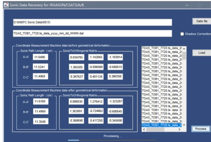
per second), not only using these equations, but also op-erating the matrixes (A3) to (A5) (see Appendix A) for Eqs. (15) and (16) along with the data of sonic paths lengths in Table A1 for Eqs. (12) and (13). Apparently, the re-covery process is a huge work load in computation. As such, these equations, matrixes, and data were implemented into a software package: “Sonic Data Recovery for IRGA-SON/CSAT3/A/B Used in Geometrical Deformation after Production/Calibration” (Appendix C and Fig. 6). As long as the path lengths and matrixes from production/calibration and from recalibration are input into the software as in-structed by the interface (Appendix C), the software auto-matically recover the data in batches.
6 Verification
In our station, an additional anemometer for wind was not under deployment when this study IRGASON was used in its deformed state; therefore, no data were available to verify the recovered 3-D wind data. However, the algorithms as ad-dressed using Eqs. (10) to (16) to recover the 3-D wind data are solid without any estimation and the recovered 3-D wind data are not necessary for verification.
Fortunately, the data to verify sonic temperature are avail-able in this station. Air temperature, relative humidity, and atmospheric pressure were measured using research grade sensors of the HMP155A and IRGASON built-in barom-eter and the data of these variables also stored at 10 Hz (10 records per second). These data can be used to esti-mate the sonic temperature (see Appendix D: Sonic tem-perature from air temtem-perature, relative humidity, and atmo-spheric pressure). The recovered data of sonic temperature using Eq. (33) were compared to the calculated sonic temper-ature over the range of sonic tempertemper-ature for three represen-tative values:−20.01±0.14◦C in Fig. 7a,−9.06±0.13◦C in Fig. 7b, and−1.90±0.22◦C in Fig. 7c. The difference between measured (i.e., unrecovered) and calculated sonic temperature values of 9.60±0.14 K in Fig. 7a, 9.53±0.17 K in Fig. 7b, and 8.93±0.24 K in Fig. 7c was narrowed to 0.99±0.14 K, 0.57±0.17 K, and −0.25±0.24 K, respec-tively, as the difference between recovered and calculated sonic temperature values. Given the accuracy of±0.5 K in sonic temperature from the IRGASON sonic anemometer (Personal communication with Larry Jacobsen, the designer of the sonic anemometer, 2017) and the accuracy of±0.2 ∼0.3 K in air temperature below 0◦C and 1.2 % in
5990 X. Zhou et al.: Recovery of the three-dimensional wind and sonic temperature data
Figure 6.Dialogue interface of software: sonic data recovery for IRGASON/CSAT3/A/B used in geometrical deformation after production and calibration.
Eq. (33) apparently did an excellent job in recovering the sonic temperature data measured using sonic anemometer in its deformed state, but was less satisfactory in the case of Fig. 7a (i.e., 0.99±0.14 K, the difference in sonic tempera-ture between recovered and calculated) although the range of 0.99±0.14 K was not significantly different from±0.80 K. The less satisfactory recovery might be caused by the ap-proximation ofc0ifromc0that is fully valid if allc0i are not measured by a sonic anemometer in its deformed state, but this is not the case in this study.
According to Eq. (22), it is impossible to have an indi-vidual c0i fromTs, which is the sole output for sonic tem-perature from any sonic anemometer. Now, the average of
c201, c022 , and c203 is known and the changes in sonic path lengths are known. It is possible to estimate the difference among the three speeds of sound and to adjust their average (c20)toc012 , c202, and c032 in approximation, although the ex-act values are impossible to determine. The adjusted values can reflect the variability amongc20i to some degree and are reasonably expected to improve the data recovery.
7 Adjustment
The measured speed of sound after crosswind correction (c0i)is independent of wind speed (Schotanus et al., 1983; Liu et al., 2001) while depending on moist air density and atmospheric pressure (Barrett and Suomi, 1949). Without wind,c0i is equal to the measured speed of sound (ci)from sonic path i(see Eq. 19). In this case, again without wind,
tui andtdi in Eq. (18) are the same and can be denoted byti.
Accordingly, Eq. (18) in this case is equivalent to
c0i≡ di
ti
. (34)
In Eq. (33),c02is the average of three squaredc0i (see Eqs. 22 and 32), but an individualc0i is unknown; therefore, for re-covery improvement, it has to be estimated fromc20through a reasonable adjustment. The difference in magnitude between
c02andc20i must be related to thec02i error due to the geomet-rical deformation of sonic anemometer. Squaring both sides of Eq. (34) leads to
c02i=d 2 i
ti2. (35)
The total differentiation ofc20i is given by
1c02i=2di
ti2 1di
−2d 2 i
ti3 1ti. (36)
Given the transmitting time is correctly measured by a sonic anemometer (i.e.,1ti=0)even in its geometrical deforma-tion, this equation becomes
1c02i=2di
ti2 1di
=c20i21di di
=c20i2(di−dT i) di
. (37)
Mathematically in differentiation,c20i can be reasonably ap-proximated byc0, given by
1c02i≈2c02
1−dT i
di
Figure 7.Verification of sonic temperature (Ts)recovered against calculated (see Appendix D) from the air temperature (T ), relative humidity
(RH), and atmospheric pressure (P )that were measured using a HMP155A air temperature and relative humidity probe as well as the IRGASON built-in barometer. Blue curves:Ts measured by the IRGASON sonic anemometer in geometrical deformation (rawTs); red
curves:Tsrecovered from rawTsusing Eq. (33); grey curves:Tsrecovered also from rawTsusing Eq. (40) (i.e., adjusted Eq. 33); and green
curves:Tscalculated fromT, RH andP.
This is the error ofc02i away fromc20. This error can be rea-sonably used to represent the deviation ofc20i away fromc02. The deviations of threec02ivalues away fromc20are the mea-sures of variability among threec20i away fromc02.
Although an individual c20i is unknown, the average of threec02i is known asc20. This average should be unchanged after adjustments because of the adjustment within the vari-ability among c02i away from c02. If the average of adjusted
c20iis not equal toc02, all adjustedc02ishould be added or sub-tracted with the same constant to make the average of three adjustedc20i values asc20, but the variability amongc20i val-ues is kept the same. This constant must be the mean of three
1c20ivalues. Based on these analyses, the adjustment ofc02to
c20ican be constructed as follows:
c20i≡c20+ 1c20i−1 3
3
X
i=1
1c02i
!
. (39)
Using this equation to replacec02iin Eq. (30) and the resultant equation with this replacement then is used for c2ci−c2i in
Eq. (27) as follows:
Tcs=Ts+ 1 3γdRd
3
X
i=1
("
c20+ 1c20i−1 3
3
X
j=1
1c02j
!
−UT2+u2T ii1d
2 T i di2
+1UcT2 −1u2cT i
)
. (40)
In the right side of this equation, the whole term afterTs is the adjusted sonic temperature recovery term.
5992 X. Zhou et al.: Recovery of the three-dimensional wind and sonic temperature data 8 Discussion
8.1 Verification of 3-D wind recovery
Although not explicitly verified, the recovered 3-D wind data were implicitly verified through the verification of recovered sonic temperature data because (1) sonic temperature is more sensitive than wind speeds in ultrasonic sonic measurements (Thomas Foken, 2018, review comment for this publication) and (2) the recovery of sonic temperature data must rely on recovered 3-D wind data (Eqs. 33 and 40). According to Eqs. (3), (17), and (21), it is apparent that sonic temperature is sensitive to one order higher than wind speed to the errors in measurements of sonic path lengths and ultrasonic signal transmitting time values. If the recovered sonic temperature is within the accuracy limits of sensors, this should be real-ized for the wind data recovery as well (Thomas Foken 2018, review comment for this publication). Additionally, the cross wind correction for sonic temperature needs 3-D wind data (Liu et al., 2001). If 3-D wind had not been well recovered, sonic temperature data could not have been recovered satis-factorily. Therefore, the satisfactory recovery of sonic tem-perature data in this study implicitly verified the satisfactory recovery of 3-D wind data.
8.2 Comparability of recovered temperature to calculated sonic temperature
The recovered sonic temperature was sourced from the mea-surements of a fast response sonic anemometer, and the cal-culated sonic temperature was sourced from the measure-ments of a slow response air temperature and relative hu-midity probe as well as a barometer built into the IRGASON (see Appendix D). Therefore, the former reflected the fluctu-ations in the sonic temperature at high frequency, and the lat-ter reflects the same fluctuations at lower frequency. As such, a pair of recovered and calculated sonic temperature values from simultaneous measurements (i.e., the same records in a time series data file) were not comparable. The difference be-tween the pair is meaningless; therefore, the mean difference between recovered and calculated sonic temperature values over a half-hour period was used for their data comparison. 8.3 Recovered temperatures higher than calculated
sonic temperature at lower temperatures
See Fig. 7. Compared to calculated sonic temperature, the recovered sonic temperature from Eq. (40) is 0.81±0.14 K higher at −20.01◦C (Fig. 7a) and 0.38±0.17 K higher at −9.06◦C (Fig. 7b); however, at −1.90◦C, even −0.45± 0.24 K lower (Fig. 7c). This trend of difference with temper-ature may be related to the performance of sonic anemome-ter at different temperature and the lower accuracy of tem-perature and humidity probe in a lower temtem-perature range (Vaisala Corp., 2017).
The sonic path lengths and geometry of the sonic anemometer were measured in the manufacture environment of an air temperature around 20◦C (i.e., manufacture
tem-perature) and embedded into its OS for field applications. However, above or below the manufacture temperature, the sonic path lengths must become, due to thermo-expansion or -contraction of sonic anemometer structure, longer or shorter than those at the manufacture temperature while the length values of sonic paths inside the OS are unchanged. As a result, the sonic anemometer could under- or overestimate the speed of sound, thus sonic temperature. The under- or overestimation may be insignificant when temperature is not much above or below the manufacture temperature while the anemometer must work best around the manufacturer temperature. In this study, the working air temperature for the sonic anemometer was as low as−20◦C, within which the sonic paths become shorter to some degree so that its measurement performance was possibly impacted. Although an assessment on the measurement performance of sonic anemometer at low or high air temperature could not be found in literature, overestimation of the speed of sound from a sonic anemometer at temperatures dozens of degrees below the manufacture temperature and thus sonic temperature is anticipated as shown in Fig. 7a to c.
However, at different air temperature the performance of the temperature and relative humidity probe and barome-ter built into the IRGASON, whose measurements are used to calculate the sonic temperature (see Appendix D), more stable than a sonic anemometer while their accuracies are the best at 20◦C and become lower with temperature away from 20◦C (Vaisala Corp., 2017). For example, HMP155A has an accuracy in air temperature to be ±0.1◦C at 20◦C
and±0.25◦C at−20◦C, as well as an accuracy in relative
humidity (RH) of ±(1.0+0.008RH) % at 20◦C and to be ±(1.2+0.012RH) % at −20◦C. The greater disagreement between recovered and calculated sonic temperature values at lower temperature in Fig. 7a may also be due to the fact that the lower the air temperature, the lower the accuracies of HMP155A and the barometer.
8.4 Radiation on calculated sonic temperature
sunlight, when such a shield was used, any heat generated from the shield under sunlight and the sensor under elec-tronic power was dissipated inefficiently (Lin et al., 2001). As a result, the air and HMP155A sensing elements inside the shield were warmer than ambient air of interest. How warm the air is inside the radiation shield depended on shield structure, ambient wind speed, and other environmental con-ditions (Blonquist et al., 2009). In the case of Fig. 7c at 750 W m−2of incoming short-wave radiation, air being a de-gree warmer inside the radiation shield was not unusual (Lin et al., 2001). In our study, this higher air temperature could directly cause the overestimation of calculated sonic temper-ature (Eq. D1 in Appendix D).
8.5 Possibility and necessity of recovering the data from a geometrically deformed sonic anemometer for fluxes
A geometrically deformed sonic anemometer outputs erro-neous data. These data may be recoverable or unrecoverable, depending on the degree of deformation. If the degree is too large, the sonic anemometer cannot perform its normal mea-surements for the transmitting time. In this case, a Camp-bell sonic anemometer sets high for one to six of its first six measurement warning flags (low amplitude, high ampli-tude, poor signal lock, large sonic temperature difference, ul-trasonic signal loss, and calibration signature error; see Ta-ble 10-2 in Campbell Scientific Inc., 2018). The geometrical deformation in sonic paths could trigger one or two flags high that indicate poor signal lock and/or ultrasonic signal loss. Regardless, in the case that any of the six warning flags from a deformed sonic anemometer were frequently, regularly, or continuously high, the erroneous data must not be recover-able (i.e., data recovery is not possible). While all six warn-ing flags are low under normal measurement conditions, the transmitting time of ultrasonic signals along each sonic path is correctly measured and the data should be recoverable. The 3-D wind data can be recovered without uncertainty although there is little uncertainty in sonic temperature (see Eqs. 33 and 40). The subsequent question is the necessity to recover the recoverable data.
A sonic anemometer is used primarily for the fluxes of mo-mentum and heat from the fluctuations in 3-D wind speeds and sonic temperature. If the fluctuations are not signifi-cantly influenced by the geometric deformation of the sonic anemometer, the data from this anemometer may not need recovering although the data are recoverable. The fluctua-tions in a wind speed component or sonic temperature are measured by variance. Therefore, this influence of sonic anemometer deformation on fluctuations in wind speed and sonic temperature can be tested through analyzing the ho-mogeneity in variance of each wind component and sonic temperature between unrecovered and recovered data.
For this study case, the 2-day data, without a missing record or any high warning flag from 10 and 11 May 2015,
were used for the analyses. After data recovery processing (Fig. 6), two datasets, unrecovered and recovered, were ac-quired. In the unrecovered dataset, for each wind speed com-ponent or sonic temperature, the data of 18 000 values from each half-hour were used to compute its variance (sk2), given by
sk2= 1 18 000
18 000
X
j=1
xkj− ¯xk
2
, (41)
wherex represents ux, uy,uz, or Ts; subscript j denotes the jth values inkth half-hour interval, and the upper bar indicates the average over the interval. In the recovered dataset, this variance was similarly computed and denoted bysRk2 , where subscript R indicates that this variance was computed from recovered dataset. For each wind component or sonic temperature, 96 variance values were available in each datasets and 192 variance values were available in both dataset. The 192 variance values for each wind component or sonic temperature can be used to construct an F-statistic (Snedecor and Cochran, 1989) to analyze the homogeneity in variance of each wind component or sonic temperature be-tween unrecovered and recovered data, given by
96
X
k=1
sk2
96
X
k=1
sRk2 ∼F (1 727 904,1 727 904). (42)
From this statistic, four F values were acquired for three wind components and sonic temperature. The four F val-ues were either > 1.00 or < 1.00, showing the inhomogene-ity in variance between unrecovered and recovered data (P< 0.001), which indicates that the geometrical deforma-tion of the sonic anemometer did significantly influence the fluctuations in each of its measured variables.
Further, using EddyPro (LI-COR Biosciences, 2016), the same datasets were used to compute two sets of sensible heat flux, latent heat flux, and CO2 flux for each half-hour in-terval. One set was computed using unrecovered data and the other set from recovered data. The two sets of flux data were shown in Fig. 8. Compared to the flux from unrecov-ered data, the flux from recovunrecov-ered data was 1.5 W m−2lower for sensible heat (P =0.031), 0.14 W m−2higher for latent heat (P =0.001), and 0.08 µmol m−2s−1 higher for CO
2 (P =0.000). These values were small in magnitude, but sig-nificant in comparison to these flux values over the ice sur-face in Antarctica.
5994 X. Zhou et al.: Recovery of the three-dimensional wind and sonic temperature data
Figure 8. Comparison of sensible heat flux, latent heat flux, and CO2flux from recovered data (red curves) to those from
unrecov-ered data (blue curves). The mean difference (the green bar rep-resents the red curve minus blue curve value) is −1.5 W m−2< 0 (P=0.031) for sensible heat flux, 0.14 W m−2> 0 (P =0.001) for latent heat flux, and 0.08 µmol m−2s−1> 0 (P=0.000) for CO2
flux.
8.6 Applicability of equations and algorithms in this study
Any sonic anemometer is slender (e.g., < 1.00 cm in each di-ameter of six claws to hold individual sonic transducers) and as light as possible to minimize its aerodynamic resistance to air flows and to maximize its stability on supporting infras-tructure (e.g., tripod) to wind momentum load, which
sacri-fices its durability in keeping its geometrical shape. There-fore, a sonic anemometer is easily deformed if not well cared for during transportation (e.g., the case in this study), instal-lation, or other handling. As shown in this study, a slight ge-ometrical deformation of sonic path length as small as mil-limeters or less (see Table A1 in Appendix A) could cause significant errors in 3-D wind and especially in sonic tem-perature. According to our recalibration experience with 3-D sonic anemometers at Campbell Scientific Inc., these cases as addressed in this study have been not unusual, but the equa-tions and algorithms to recover the data measured by a de-formed 3-D sonic anemometer were not available. As requi-sitions of these datasets are expensive, their recovery would be a cost-effective and time-saving option.
The equations and algorithms in this study were developed based on the measurement working physics and sonic path geometry of the IRGASON sonic anemometer. The physics is the same as those for other models of Campbell Scientific 3-D sonic anemometers in use, such as CSAT3, CSAT3A, and CSAT3B (Campbell Scientific Inc., UT, USA; Horst et al., 2015). However, the sonic path geometry of the IRGA-SON sonic anemometer is different from other models in the assigned azimuth angle of the first sonic path in the 3-D anemometer coordinate system. This angle was assigned as 90◦ in the IRGASON sonic anemometer, but as 0◦ in other models (e.g., CSAT3, CSAT3A, and CSAT3B). Even so, given the sonic path lengths and transfer matrixes of sonic anemometer that were measured and determined in the man-ufacture or calibration process (di in Eq. 12 andAin Eq. 15) and in the recalibration process after use in the geometri-cal deformation state (dT i in Eqs. 13, 33, and 40 and AT in Eqs. 14 and 16), the equations and algorithms from this study are applicable to all models of Campbell Scientific 3-D sonic anemometers (Fig. 6) except for CSAT3 if its bugged OS version 4 is used (Burns et al., 2012). The derivation pro-cedures and even equations based on the measurement work-ing physics are applicable as a reference to the development of the equations and algorithms to recover the data measured using other brands of 3-D sonic anemometers that incurred deformations or to studies on similar topics.
9 Conclusion remarks
tempera-ture data measured by this sonic anemometer in its deformed state before the recalibration, equations and algorithms were developed and implemented into a software package: “Sonic Data Recovery for IRGASON/CSAT3/A/B Used in Geomet-rical Deformation after Production/Calibration” (Fig. 6 and Appendix C). Given two sets of sonic path lengths and two transfer matrixes of sonic anemometer that were measured and determined in the manufacture and calibration process and also in recalibration process after the use in its de-formed state, the data measured by the IRGASON 3-D sonic anemometer, even in its deformed state, were recovered as if measured by the same anemometer recalibrated immediately after its deformation.
Inside a Campbell Scientific sonic anemometer, the transducer-shadow correction for 3-D wind (Wyngaard and Zhang, 1985) is an available, programmable option for a user. However, the crosswind correction for sonic tempera-ture (Liu et al., 2001) is internally applied as default by its OS. In a case of transducer-shadow correction in option, the 3-D wind data are recovered using Eqs. (10) to (16). If not, Eqs. (15), (12), (13), and (16) are sequentially used. Based on the data from the recovery process of 3-D wind, the sonic temperature data are recovered using Eqs. (9), (32), (38), and (40); therefore, the satisfactory recovery for both 3-D wind data and sonic temperature can be eventually reflected by the satisfactory of sonic temperature data recovery.
The software based on the equations and algorithms from this study can recover the 3-D wind data with or without the transducer-shadow correction inside the sonic anemometer and sonic temperature data with crosswind correction also inside the sonic anemometer. It was verified by comparing the recovered to calculated sonic temperature data (Appendix D). As shown in Fig. 7, the recovered data of sonic temper-ature using Eqs. (33) and (40) were compared to the calcu-lated sonic temperature of three representative values over the range of measured sonic temperature from −20.01 to −1.90◦C. The difference of 9.60 to 8.93 K between unrecov-ered and calculated sonic temperature (i.e., unrecovunrecov-ered mi-nus calculated) was narrowed by Eq. (40) to 0.81 to−0.45 K (i.e., recovered minus calculated), which was satisfactory for measurements of sonic anemometer below 0 to−20◦C. Af-ter verification, the software was used to recover the data measured by the IRGSON (SN: 1131) 3-D sonic anemome-ter in its deformed state from May 2015 to January 2016. The 8-month data were recovered using 3 days of one engineer’s time. Further, using EddyPro 6.2.0 (LI-COR Inc., 2016), the recovered data were processed for the fluxes of CO2/H2O, sensible heat, and momentum. The data quality (Foken et al., 2012) mostly ranged in 1 to 3 and the energy closure with-out considering surface heat flux into ice were > 83 % when friction velocity was > 0.2 m s−1. Although energy balance closure is not a good indicator for data quality (Foken et al., 2012), this closure rate is fair.
The use of a deformed 3-D sonic anemometer is a prac-tical case. The analyses of our study case indicated that the measured fluctuations in wind speeds and sonic temperature as well as fluxes were significantly influenced by the defor-mation. If the data from such a use cannot be recovered, the requisition of these data is expensive and their recovery would be a cost-effective and time-saving option. The equa-tions, algorithms, and software are applicable to all models of Campbell Scientific 3-D sonic anemometers such as CSAT3, CSAT3A, and CSAT3B that are used around the world. The derivation procedures and even equations based on the mea-surement working physics of sonic anemometers are appli-cable as a reference to the development of the equations and algorithms to manage the data measured using other brands of 3-D sonic anemometers or recover the data measured by an anemometer in its deformed state.
5996 X. Zhou et al.: Recovery of the three-dimensional wind and sonic temperature data Appendix A: Transform matrixes
In micrometeorological applications, the wind speeds are ex-pressed in a three-dimensional (3-D) orthogonal coordinate system of anemometer or natural wind, but a sonic anemome-ter measures flow velocities along its three non-orthogonal sonic paths (i.e., situated non-orthogonally from each other, see Figs. 1 and A1); therefore, for applications, the flow ve-locities along the three sonic paths need to be transformed into a 3-D right-handed orthogonal coordinate system in ref-erence to the geometry of sonic anemometer, as shown in Fig. A1 (i.e., the 3-D orthogonal anemometer coordinate sys-tem). Givenuxanduy are two horizontal velocities in thex and y direction, respectively, anduz is vertical velocity in thezdirection (Fig. A1);x,y, andzare the three coordinate axes in the 3-D orthogonal anemometer coordinate system. This system is defined with the x–y plane, parallel to the anemometer bubble-leveled plane, with the first sonic path on they–zplane, and with origin in the center of measure-ment volume. A flow speed along theith (i=1,2, or 3) sonic path is a combination of component velocities ofux,uy, and uz; given by
ui= uxcosφi+uysinφisinθi+uzcosθi, (A1) whereθi andφi are the zenith and azimuth angles of theith sonic path in the 3-D orthogonal anemometer coordinate sys-tem. In this system (see Fig. A1), given the first sonic path has an azimuth angle ofφ1equal to 90◦as fixed on thex−y plane, Eq. (A1) can be expressed in a matrix form of
u1
u2
u3
=
0 sinθ1 cosθ1
sinθ2cosφ2 sinθ2sinφ2 cosθ2 sinθ3cosφ3 sinθ3sinφ3 cosθ3
ux uy uz
=A
−1
ux uy uz
, (A2)
where A is a matrix expressing the flow speeds along the three non-orthogonal sonic paths in the 3-D orthogo-nal anemometer coordinate system. Nomiorthogo-nally for the sonic paths of the IRGASON, θ1, θ2, and θ3 are all 30◦ and φ2 andφ3 are 330 and 210◦, respectively (see Fig. A1). Given
φ1=90◦, these angles are calculated using measured data from a coordinate measurement machine and, along with the sonic path lengths, are listed in Table A1 for the IRGASON serial no. of 1131 before and after its geometrical deforma-tion.
Using the data in this table, matrixAin Eq. (A2) and its inversionA−1for this IRGASON before its geometric defor-mation (i.e., as used in the IRGASON OS but not valid in the field after deformation) are given as follows:
A=
0.034785 1.142665 −1.183914 1.365505 −0.696580 −0.660515 0.367627 0.401124 0.380356
, (A3)
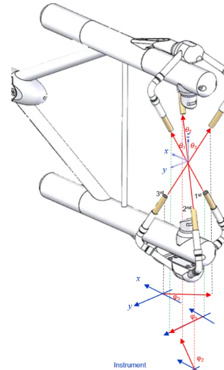
Figure A1.IRGASON sonic path angle geometry in the three-dimensional right-handed anemometer coordinate system ofx,y, andz. Blue arrows are coordinates; a red arrow between a pair of sonic transducers is the sonic path vector whose direction is defined for air flow direction, the red arrow below the IRGASON is the projection of the corresponding sonic path vector on thex–yplane, i.e., anemometer (instrument) bubble-leveled plane. As indicated by their subscript of 1, 2, or 3 for the first, second, or third sonic path,
θ1,θ2, andθ3are their zenith angles andϕ1,ϕ2, andϕ3are their
azimuth angles.
and
A−1=
0.00000 0.499023 0.866589 0.418196 −0.246062 0.874394 −0.441030 −0.222826 0.869391
. (A4)
After the IRGASON geometrical deformation, matrixA be-came
AT=
0.006035 1.276412 −1.323287 1.363991 −0.724862 −0.600545 0.368690 0.417250 0.345690
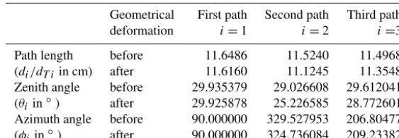
Table A1.The lengths, zenith angles, and azimuth angles of sonic paths in the IRGASON (serial no.: 1131) anemometer coordinate system before and after its geometrical deformation (measured using a coordinate measurement machine on 9 September 2014 before the deforma-tion and on 6 March 2016 after deformadeforma-tion).
Geometrical First path Second path Third path deformation i=1 i=2 i=3 Path length before 11.6486 11.5240 11.4968 (di/dT iin cm) after 11.6160 11.1245 11.3548
Zenith angle before 29.935379 29.026608 29.612041 (θiin◦) after 29.925878 25.226585 28.772601
Azimuth angle before 90.000000 329.527953 206.80477 (φi in◦) after 90.000000 324.736084 209.23382
where subscript T indicates “True” because, after the IRGA-SON deformation, it should be used in the field although it was not used. The inversion of this matrix is given as follows:
A−T1=
0.000000 0.498879 0.866672 0.347992 −0.246063 0.904629 −0.420029 −0.235072 0.876537
. (A6)
MatrixesA−1,AT, andA−T1were used for our data recovery andAwas also used in the sonic anemometer OS.
Appendix B: Iteration algorithm for sonic transducer-shadow corrections
Given transform matrixA, using Eq. (5), the measured wind vector [u1 u2 u3]0along the sonic paths is transformed to the wind vector in the 3-dimensional orthogonal anemometer coordinate system
ux uy uz0. Subsequently,UTis cal-culated using Eq. (9). ReplaceuT iwithui under the square root in the right side of Eq. (8), an approximate equation for the first iteration is given as follows:
uT i_1≈
ui
0.84+0.16 q
UT2−u2i UT
, (B1)
whereiis 1, 2, or 3 and subscript 1 ofuT iindicates that it is calculated from the first iteration.
First iteration
Equation (B1) is used for sonic transducer-shadow correc-tions in the first iteration.
Second iteration
ux uy uz
=A
uT1_1
uT2_1
uT3_1
(B2)
Using Eq. (9),UT is recalculated. Replaceui withuT i_1 under the square root in the right side of Eq. (B1), an approx-imate equation for the second iteration is given as follows:
uT i_2=
ui
0.84+0.16 q
U2 T−u2T i_1
UT
(B3)
Third iteration . . .
nth iteration
ux uy uz
=A
uT1_m uT2_m uT3_m
(B4)
where subscriptm=n−1. Using Eq. (9),UTis also recalcu-lated. Similar to the calculation foruT i_2,uTi_nis calculated using the following equation:
uTi_n=
ui
0.84+0.16 q
U2 T−u2T i_m
UT
, (B5)
to ensure that the difference inux,uy, oruzbetween the last and previous iterations is<1 mm s−1≈1.96σ, where σ is the maximum precision (i.e., standard deviation at constant wind) amongux,uy, anduz(Campbell Scientific Inc., 2018). Our numerical tests within the measurement ranges inux, uy, anduzconcluded that the iterations mostly converged at n=2 and entirely atn≤3.
Appendix C: MATLAB code
5998 X. Zhou et al.: Recovery of the three-dimensional wind and sonic temperature data Note: This code can be compiled in MATLAB as an
executable file: Data_recovery.exe.
% sonicdatarecovery Sonic Data Recovery for IRGA-SON/CSAT3/A/B Used in Geometrical Deformation after Production/Calibration
%Syntax:
function [Ux,Uy,Uz,Ts,Ts1,Ts2,Raw]= sonicdatarecovery(RAW)
% Inputs:
% um Measured 3-D wind speeds in the orthogonal anemometer coordinate system (OCS)
%TsMeasured sonic temperature
%AMatrix of sonic to OCS before geometrical deforma-tion
%ATMatrix of sonic to OCS after geometrical deforma-tion
% di Sonic path length before geometrical deformation (i=1, 2, or 3)
% dTi Sonic path length after geometrical deformation (i=1, 2, or 3)
% Constants
shadow_correction_flag =1; % %Shadow correction has been done (=1) or not (=0) inside OS
gama_d=1.4003; %% the ratio of dry air specific heat at constant pressure to that at constant volume
Rd=287.04; %% gas constant for dry air
RV=4.61495e−4; %% gas constant for water vapor Av=60.064621; Bv=60.973392; Cv=60.387959; Ah=0.000000; Bh=59.527953; Ch=63.195226;
Avt=60.074122; Bvt=64.773415; Cvt=61.227399; Aht=0.000000; Bht=54.736084; Cht=60.766176; % Browse to the raw data file directory to load files in a batch
hwait=waitbar(0,“Please select the file to be processed”); pause(0.5)
[name,path]=uigetfile(“*.*”,“stabilitylect a folder”); fname=[path name];
close(hwait);
RAW=dlmread(fname,’,’, 4, 1);
% Extract sonic anemometer and other meteorological data
UX=RAW(:,2); UY=RAW(:,3); UZ=RAW(:,4); TRAW=RAW(:,5); H2O=RAW(:,8);
Temp=RAW(:,10); P=RAW(:,11); amb_e=RV.*H2O.*(Temp+273.15);
TS_emp=(Temp+273.15).*(1+0.32*amb_e./P)−273.15;
% Load transform matrix of Eq. (A2) and data of Table A1 before geometrical deformation
The1=((90-Av)/180)*pi; The2=((90-Bv)/180)*pi; The3=((90-Cv)/180)*pi;
Phi1=((90-Ah)/180)*pi; Phi2=((270+Bh)/180)*pi; Phi3=((270-Ch)/180)*pi;
A_inversion=[0 sin(The1) cos(The1);
sin(The2)*cos(Phi2) sin(The2)*sin(Phi2) cos(The2); sin(The3)*cos(Phi3) sin(The3)*sin(Phi3) cos(The3)]; A=A_inversion(−1);d= [11.6486;11.5240;11.4968]; % Load transform matrix of Eq. (A5) and data of Table A1 after geometrical deformation
The1=((90-Avt)/180)*pi; The2=((90-Bvt)/180)*pi; The3=((90-Cvt)/180)*pi;
Phi1=((90-Aht)/180)*pi; Phi2=((270+Bht)/180)*pi; Phi3=((270-Cht)/180)*pi;
AT_inversion=[0 sin(The1) cos(The1);
sin(The2)*cos(Phi2) sin(The2)*sin(Phi2) cos(The2); sin(The3)*cos(Phi3) sin(The3)*sin(Phi3) cos(The3)];
AT=AT_inversion∧(-1); dT=[11.6159;11.1245;11.3548];
% Prompt data processing is in progress hwait=waitbar(0,“Processing> > > > > > ”) %Recover 3-D wind data
%Get measured flow speeds along each of 3 sonic paths [mRaw,nRaw]=size(RAW);
fori=1:mRaw;
um=[UX(i);UY(i);UZ(i)];
%With transducer-shadow corrections (TSC):
UT=(um(1)2+um(2)∧2+um(3)∧2)∧(1/2); %% Calculate the total wind magnitude
if isequal(shadow_correction_flag, 1) %% TSC has been done (=1) inside firmware
u=A_inversion*um; %% Calculate the vector of the three flow speeds using Eq. (10)
ut1(1)=u(1)/(0.84+0.16.*((UT∧2-u (1)∧2)∧(1/2))./UT);
%% Eq. (11), recover flow speed along sonic path 1 before TSC
ut2(1)=u(2)/(0.84+0.16.*((UT∧2-u (2)∧2)∧(1/2))./UT);
%% Eq. (11), recover flow speed along sonic path 2 before TSC
%% Eq. (11), recover flow speed along sonic path 3 before TSC
uc=[ut1.*(dT (1)./d(1));ut2.*(dT(2)./d(2));ut3. *(dT(3)./d(3))]; %% Eq. (13)
uts1=ut1; uts2=ut2; uts3=ut3; %%Corrected 3-D wind speed um_c=AT*uc; %% Eq. (16)
%Iteration algorithm of sonic TSC (Appendix B) for recovered data
UT_C=(um_c (1)∧2+um_c ()∧2+um_c (3)∧2)∧(1/2); %% Total wind magnitude
% 1st iteration
uct1=uc (1)/(0.84+0.16.*((UT∧2-uc (1)∧ 2)∧(1/2))./UT); % %flow speed 1
uct2=uc (2)/(0.84+0.16.*((UT∧2-uc (2)∧
2)∧(1/2))./UT); % %flow speed 2
uct3=uc (3)/(0.84+0.16.*((UT∧2-uc (3)∧ 2)∧(1/2))./UT); % %flow speed 3
% 2nd iteration
for q=2:5; %% 5 steps of iterations after 1st iteration are adequate
%TSC for flow speed 3
uct_m=[uct1(q-1);uct2(q-1);uct3(q-1)]; %% Vector of three path flow speeds
um_C=AT*uct_m; %%Vector in 3-D orthogonal system UT_C=(um_C (1)∧2+um_C (2)∧2+um_C
(3)∧2)∧(1/2);
%% Total wind magnitude, again
uct3(q)=uc (3)/(0.84+0.16.*((UT_C∧2-uct3
(q-1)∧2)∧(1/2))./UT_C);
%% TSC for flow speed 3 % TSC for flow speed 2
uct_mm=[uct1(q-1);uct2(q-1);uct3(q)]; %%Vector of three flow speeds, again
um_C=AT*uct_mm; %% Vector in 3-D orthogonal sys-tem, again
UT_C=(um_C (1)∧2+um_C (2)∧2+um_C
(3)∧2)∧(1/2); %% Recalculated the total wind magnitude uct2(q)=uc (2)/(0.84+0.16.*((UT_C∧2-uct2
(q-1)∧2)∧(1/2))./UT_C); %%% TSC for flow speed 2 %TSC for flow speed 1
uct_mm=[uct1(q-1);uct2(q);uct3(q)]; %%Vector of three flow speeds, again
um_C=AT*uct_mm; %% Vector in 3-D orthogonal sys-tem
UT_C=(um_C (1)∧2+um_C (2)∧2+um_C (3)∧2)∧(1/2); %% Total wind magnitude, again uct1(q)=u (1)/(0.84+0.16.*((UT_C∧2-uct1 (q-1)∧2)∧(1/2))./UT_C); %%%TSC for flow speed 1
% Judge the steps of iterations
uct_n=[uct1(q);uct2(q);uct3(q)]; %%Vector from current iteration
ABS_C=uct_n-uct_m; %%Difference between two iter-ations
% Exit condition
if(abs(ABS_C(1))< =0.001&&abs(ABS_C(2))< =0.001&&abs(ABS_C(3))<=0.001);
%Finalize recovered 3-D wind speed ucm=AT*uct_n; %% Eq. (14)
ucts1=uct1(q); ucts2=uct2(q); ucts3=uct3(q); break; %% %Exit iterations
end end else
%Recover 3-D wind data without TSC
u=A_inversion*um; %% Acquire the flow speeds along 3 sonic paths, Eq. (10)
uc=[dT(1)./d(1).*u(1); dT(2)./d(2).*u(2); dT(3)./d(3).*u(3)]; %%Correction
ucm=AT*uc; %%3-D orthogonal data after recovery uts1=uc(1); uts2=uc(2); uts3=uc(3);
ucts1=ucm(1); ucts2=ucm(2); ucts3=ucm(3); end
%Recover sonic temperature data Ts=TRAW(i);
UcT= (ucm (1)∧2 + ucm (2)∧2 + ucm (3)∧2)∧(1/2); %% Total wind
C02 = gama_d*Rd*(Ts+273.15); %% Eq. (32) DELTUcT2 = UcT∧2 – UT∧2;
DELTucT21 =ucts1∧2 – uts1∧2; DELTucT22=ucts2∧2
– uts2∧2; DELTucT23=ucts3∧2 – uts3∧2;
DELTC21=(C02 - UT∧2+uts1∧2)*((dT(1)∧2 – d(1)∧2)/d(1)∧2); %% Eq. (30)
DELTC22=(C02 - UT∧2+uts2∧2)*((dT(2)∧2 – d(2)∧2)/d(2)∧2); %% Eq. (30)
DELTC23=(C02 – UT∧2+uts3∧2)*((dT(3)∧2 – d(3)∧2)/d(3)∧2); %% Eq. (30)
AAA=(DELTC21+DELTUcT2 – DELTucT21); BBB=(DELTC22+DELTUcT2 – DELTucT22); CCC=(DELTC23+DELTUcT2 – DELTucT23); DDD=(AAA+BBB+CCC);
EEE=3*gama_d*Rd;
Tcs=Ts+(DDD/EEE); %% Eq. (33)
DELTC021_ad=C02*2*(1-dT(1)/d(1)); %% Eq. (38) DELTC022_ad=C02*2*(1-dT(2)/d(2)); %% Eq. (38) DELTC023_ad=C02*2*(1-dT(3)/d(3)); %% Eq. (38) AAA_ad=((dT(1)∧2-d(1)∧2)/d(1)∧ 2)*(C02-(DELTC021_ ad+((DELTC021_ad+DELTC022_ ad+ DELTC023_ad)/3))-UT∧2+uts1∧2)
+DELTUcT2-DELTucT21;
BBB_ad=((dT(2)∧2-d(2)∧2)/d(2)∧2)