Page 319 www.ijiras.com | Email: [email protected]
Implementation Of Maximum Power Point Tracking With A Boost
Converter And A Three Level 3-Phase Inverter Connected To The
Grid
Noumsi Damien Brice
Engr. Dr. Nentawe Y. Goshwe
Manji Y. Morkat
Department of Electrical/Electronics Engineering, University of Agriculture, Makurdi, Benue State, Nigeria
I. INTRODUCTION
In today‘s world, renewable energy sources play important role in electricity generation. Several sources like wind, solar, biogas etc. are important energy sources. Energy from the sun is the best option for renewable energy as it is available almost everywhere and is free to harness [1]-[2]. Solar radiation from the sun is converted to electrical energy by using solar cells which exhibit photovoltaic (PV) effect. However, for PV systems, the amount of electric power generated changes continuously with weather conditions.
For solar to be a competitive energy source it is extremely important to extract the maximum power from each panel and lower the cost per kilowatt. It turns out that this is not as simple as just hooking a panel to a battery or grid; there are many variables that affect the performance of a panel, such as shade, shadows, and ambient temperature—thus the need for MPPT algorithms. Solar cells, like other silicon diodes, have an exponential transfer function from voltage to current. A small change in voltage results in a large change in current. Two important factors that have to be taken into account are the irradiation and the temperature. In general, I-V curve for a PV array is non – linear so a specific point on the curve
Abstract: The power output of the solar array is dependent of the irradiance, temperature and internal properties of the materials used to make solar cells. These factors contribute in the position of the Maximum power point. Changes in atmospheric conditions affect directly the output of the solar panel. Therefore, there is a need to track the Maximum power point to ensure that the system delivers the maximum power and the losses are reduced at any given time despite the change in temperature and irradiation throughout a day. The maximum power point tracking(MPPT) of the PV output for all sunshine conditions is a key to keep the output power per unit cost low for successful PV applications. Several techniques have been proposed for maximum power point tracking. The most commonly used technique for MPPT is the perturb and observe technique. MATLAB was used to simulate the Perturb and observe. The main aim will be to track the maximum power point of the photovoltaic module so that the maximum possible power can be extracted from the photovoltaic. The algorithms utilized for MPPT are generalized algorithms and are easy to model or used as a code. The algorithms are written in m files of MATLAB and utilized in simulation where the values of the irradiance and temperature were chosen based on the average values in Benue State. The solar cell is modeled using SIM Power Systems blocks.
Page 320 www.ijiras.com | Email: [email protected] namely maximum power point needs to be tracked so that the
whole system operates at maximum efficiency and produces maximum output power. Hence, Maximum Power Point Tracking (MPPT) algorithm is used for extracting maximum power available from a PV module under different conditions. Out of numerous available techniques the one that is used most widely and commonly is Perturb & Observe (P&O) algorithm. P&O is also called as hill climbing method because it checks the rise of the curve till MPP and the fall after that point[3]-[8]. Using P&O algorithm the controller adjust voltage and measures power and if this measured power is greater than the previous value of power, adjustments are made in the same direction until there is no more increment in power.
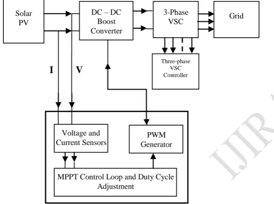
Generally, the MPPT controller is embedded in the power electronic converter systems, so that the corresponding optimal duty cycle is updated to the photovoltaic power conversion system to generate the maximum power point output.
I V
Figure 1: Block diagram of the proposed system
II. THE SOLAR CELL
The solar cell is the basic building block of solar photovoltaic. The cell can be considered as a two terminal device which conducts like a diode in the dark and generates a photo voltage when charged by Sun[9]. When charged by the Sun, this basic unit generates a dc photo voltage of 0.5 to 1volt and in short circuit, a photocurrent of some tens of miliamperes per cm2.
Figure 2: Equivalent circuit of PV solar cell
PV arrays are built up with combined series or parallel combinations of PV solar cells, which are usually represented by a simplified equivalent circuit model such as the one given in Figure2 and/or by an equation as in (1).
h
R
I
R
V
nKT
I
R
v
q
I
I
I
s s s
ph
1
(
exp
0 (1)
The output characteristic of a photovoltaic (PV) array is non-linear and is influenced by solar irradiance level, ambient temperature, wind speed, humidity, pressure, etc. The irradiation and ambient temperature are the two primary factors. To study the output characteristics of PV cell, some experiments based on simulation of PV cell have been done.
For constant temperature (25˚C) and different intensity (400-1000W/m2) The PV array current constant up to some voltage level and then it will be decreased. The PV array current always increases with intensity.
THE BOOST CONVERTER
The boost converter was chosen for its benefits in terms of cost saving, simplicity and efficiency. The values of some components such as inductor and capacitor were determined by using suitable equations in order to make sure continuous conduction mode is sustained.
Figure 3 depicts the basic circuit of an ideal boost converter with Vd and Vo as input and output voltages
respectively and figure 4 shows the waveforms of the boost converter.
Figure 3: Ideal boost converter
Figure 4: The waveforms of Boost Converter
Solar PV
Three-phase VSC Controller
DC – DC Boost Converter
3-Phase
VSC Grid
Voltage and Current Sensors
PWM Generator
Page 321 www.ijiras.com | Email: [email protected] There are two modes of operation of a boost converter.
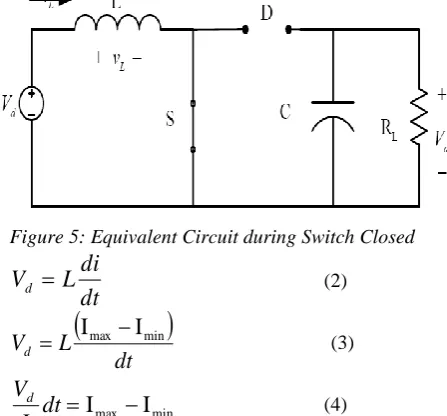
The operation mainly based on the ON and OFF mode of the switch. Firstly, when the switch is closed, this can be known as charging state. After that, second mode of operation will be initiated by opening the switch, and this state is known as discharging mode of operation.
Figure 5: Equivalent Circuit during Switch Closed
dt
di
L
V
d
(2)
dt
L
V
d min maxI
I
(3)min max
I
I
dt
L
V
d (4)dt
L
V
d
min maxI
I
(5)During discharging mode of operation, the switch is open and the diode is forward biased, as shown in Figure 6. At this time, the inductor is discharged to the capacitor and meets the load demand.
Figure 6: Equivalent Circuit during Switch Opened
d
I
I
V
V
d
0 (6))
2
D
(Since
2
)
(
L
2f
f
Rd
d
I
(7)Rcf
d
V
V
O
0 (8)dT
0R
V
V
C
o
(9)VSC CONVERTER
The proposed inverter structure is designed to make use of a three-level topology called neutral point clamped. The IGBT semiconductor is used due to its lower switching losses
and reduced size when compared to other power electronic devices. Indeed, the control of the output voltage is provided by the PWM technique. The three-level VSC regulates DC bus voltage at 500 V and keeps unity power factor. Id current reference is the output of the DC voltage external controller. Iq current reference is set to zero in order to maintain unity power factor. Vd and Vq voltage outputs of the current controller are converted to three modulating signals Uref_abc used by the PWM three-level pulse generator. The control system uses a sample time of 100 μs for voltage and current controllers. In the detailed model, pulse generators of Boost and VSC converters use a fast sample time of 1μs in order to get an appropriate resolution of PWM waveforms.
Figure 7: 3-Level Inverter
The inverter block implements a 3-level three-phase power converter that consists of up to six power switches connected in a bridge configuration. The type of power switch and converter configuration is selectable from the dialog box. The block allows simulation of converters using either naturally commutated (or line-commutated) power electronic devices (diodes or thyristors) and forced-commutated devices (GTO, IGBT, MOSFET).
SWITCHING TABLE
The switching table is formed using the sector, the corresponding voltage vector and the switch state. The summary of various states are given in table 1.
Table 1: 3 Level Inverter Switching Table
State No.
SwitchingStates
Vab Vbc Vca
S1 S2 S3 S4 S5 S6
1 ON ON OFF OFF OFF ON VS 0 -VS
2 ON ON ON OFF OFF OFF 0 VS -VS
3 OFF ON ON ON OFF OFF -VS VS 0
4 OFF OFF ON ON ON OFF -VS 0 VS
5 OFF OFF OFF ON ON ON 0 -VS VS
6 ON OFF OFF OFF ON ON VS -VS 0
7 ON OFF ON OFF ON OFF 0 0 0
Page 322 www.ijiras.com | Email: [email protected] III. MPPT ALGORITHM: PERTURB AND OBSERVE
METHOD (P&O)
This method is one of the simplest online methods which, has been considered by a number of researchers [10–17]. P&O can be implemented by applying perturbations to the reference voltage or the reference current signal of the solar panel. A flowchart illustrating this method, which is also known as the ‗hill climbing method‘ is depicted in Figure 7, where ‗‗V‘‘ is the reference signal. In this algorithm, if the reference signal, V is taken as the voltage, the goal will involve pushing the reference voltage signal towards VMPP thereby causing the
instantaneous voltage to track the VMPP. As a result the output
power will approach MPP. To this end, a small but constant perturbation is applied to the solar panel voltage. The solar panel voltage is changed by applying a series of small and constant perturbations denoted by (C=∆V) on a step-by-step basis in order to change the system operating point. Following each perturbation, the output power variation (∆P) is measured. If ∆P is positive, power will approach MPP, therefore a voltage perturbation of the same sign must be applied in the following stage. A negative ∆P, on the other hand, implies that power has moved away from MPP, and a perturbation of opposite sign will have to be applied. This process is repeated until the MPP is reached.
Figure 8: Conventional Perturb and Observe algorithm
Figure 9: Proposed circuit diagram
IV. RESULTS
A. SIMULATION OF TEMPERATURE AND
IRRADIATION
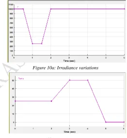
Figure 10 shows the irradiance and temperature variations generated as inputs on the solar array. Figure 10a shows irradiance generated at a constant value of 1000Kw/m2for 0.5 second, decreases at 250Kw/m2 for 0.5 second. The system increases steadily from 250Kw/m2 at 0.5seconds to 1000Kw/m2 at 2 seconds and is maintained constant.
Figure 10b shows a simulated behavioural pattern of temperature variation on the PV module. At a temperature of 250C (room temperature) for a period of 2 seconds, the PV module output varies as its temperature increases to an extreme value of 500C.
Figure 10a: Irradiance variations
Figure 10b: Temperature variations
B. RESULT FROM THE SOLAR PANEL
Page 323 www.ijiras.com | Email: [email protected]
D
uty
cycl
e
Cur
re
n
t
Vol
tag
e
Duty c
yc
le
Curr
en
t
Volta
ge
Figure 11 (b): P-V characteristics of Sola array for various irradiance at a constant temperature of 250C
For constant temperature (25˚C) and different intensity (400- 1000W/m2), the PV array power increases up to some voltage level and then it will be decreased. The PV array power always increases from low to high intensity.
Figure 12 (a): I-V characteristics of Solar array for various temperature at constant irradiance of 1000W/m2
Figure 12 (b): P-V characteristics of Solar array for various temperature at a constant irradiance of 1000W/m2
C. RESULTS FROM THE BOOST CONVERTER
OUTPUT
Figure 13 shows the duty cycle of the DC converter over a period of 5.5seconds which also varies a lot as the irradiance and temperature are varied.
Figure 14 displays the waveform of the current output of the DC converter over a period of 5.5seconds using the same variations in the irradiance and temperature. The current also varies with the duty cycle. The system has a dynamic performance as it can be noted as it has a quick rise time as the duty cycle also rises.
Figure 15 shows the voltage output of the DC converter over a period of 5.5seconds using the conventional technique
with the same variations in the input parameters. The voltage curve also shows that the voltage decreases as the duty cycle changes.
Figure 16 shows the power output of the DC converter over a period of 5.5seconds using the conventional technique with the irradiance and temperature varied. By adjusting the voltage different output curves can be obtain with different steady state response and rise time.
Figure 13: Duty cycle using the conventional MPPT
Figure 14: current output using the conventional MPPT
Page 324 www.ijiras.com | Email: [email protected]
P
o
wer
Mo
d
u
lation
P
o
wer
Cur
re
n
t
Vol
tag
e
Pow
er
Volta
ge
Curr
en
t
Pow
er
Figure 16: Power output using the conventional MPPT
D. RESULTS FROM THE VOLTAGE SOURCE
CONVERTER
a. RESULTS FROM THE VOLTAGE SOURCE
CONVERTER USING THE CONVENTIONAL
PERTURB AND OBSERVE TECHNIQUE
Figure 17 shows the voltage of the VSC using the conventional perturb and observe technique as the irradiance and temperature are varied.
Figure 18 shows the current output of the VSC using the conventional perturb and observe technique; as the input parameters (irradiance and temperature) are varied, changes are also observed.
Figure 19 shows the power output of the VSC where many oscillations are observed and also the hill climbing problem is glaring. The curve also exhibits changes as the input parameters are varied.
Figure 20 shows the modulation index of the VSC as it varies with the input parameters.
Figure 17: Voltage output of the VSC
Figure 18: Current output of the VSC
Figure 19: Power output of the VSC
Figure 20: Modulation Index
V. CONCLUSIONS AND RECOMMENDATIONS
Page 325 www.ijiras.com | Email: [email protected] of PV panel working with a connected load. It also gives an
advantage of pre evaluating overall system before going into real time. The whole PV panel – MPPT – Grid tied system is created in MATLAB/Simulink. PV panel Simulink block has under gone I-V, P-V characteristic check and results are obtained.
Further work is required to address some shortcomings of the algorithm. The original basis for the algorithm was the Perturbation and Observation technique which means that it may suffer from tracking in the wrong direction under rapidly changing conditions. Further work is also required into the methods used to select the best combination of parameters for the algorithm.
REFERENCES
[1] B. K. Bose, ―Energy, environ ment, and advances in power electronics,‖ IEEE Trans. Power Electron., vol. 15, no. 4, pp. 688-701, Jul. 2000.
[2] F. Blaabjerg, C. Zhe, and S. B. Kjaer, ―Po wer e lectronics as efficient interface in dispersed power generation systems,‖ IEEE Trans. Power Electron., vol. 19, no. 5, pp.1184-1194, Sep. 2004.
[3] T. Esram and P. L. Chap man, ― Comparison of photovoltaic array maximum power point tracking techniques,‖ IEEE Trans. Energy Convers., vol. 22, no. 2, pp. 439–449, Jun. 2007.
[4] V. Salas, E. Olias, A. Barrado, and A. La zaro, ― Review of the maximum power point tracking algorithms for standalone photovoltaic systems,‖ Sol. Energy Mater. Sol.
Cells, vol. 90, no. 11, pp. 1555–1578, Jul. 2006.
[5] G. Petrone, G. Spagnuolo, R. Teodorescu, M. Veerachary, and M. Vitelli, ―Re liability issues in photovoltaic power processing systems,‖ IEEE Trans. Ind. Electron., vol. 55, no. 7, pp. 2569–2580, Jul. 2008.
[6] C. Hua, J. Lin, and C. Shen, ―Imp lementation of a DSPcontrolled photovoltaic system with peak power trac king,‖ IEEE Trans. Ind. Electron., vol. 45, no. 1, pp. 99– 107, Feb. 1998.
[7] T. Noguchi, S. Togashi, and R. Nakamoto, ―Short -current pulse-based maximum-power-point tracking method for multiple photovoltaic-and converter module system,‖
IEEE Trans. Ind. Electron., vol. 49, no. 1, pp. 217–223,
Feb. 2002.
[8] N. Mutoh, M. Ohno, and T. Inoue, ―A method for MPPT control while searching for parameters corresponding to weather conditions for PV generation systems,‖ IEEE
Trans. Ind. Electron., vol. 53, no. 4, pp. 1055– 1065, Jun.
2006.
[9] Surya Kumari J., Ch. Sai Babu2 and J. Yugandhar3 ―Design and Investigation of Short Circuit Current Based Maximum Power Point Tracking for Photovoltaic system‖, International Journal of Research and Reviews in Electrical and Computer Engineering (IJRRECE) Vol. 1, No. 2, June2011.
[10]Wasynczuk O. Dynamic behavior of a class of photovoltaic power systems. IEEE Transactions on Power Applications System 1983; 102(9):3031–7.
[11]Hua C, Lin JR. DSP-based controller application in battery storage of photo- voltaic system, In: Proc. IEEE IECON 22nd Int. Conf. Ind. Electron., Contr. Instrum.; 1996, pp. 1705–1710.
[12]Slonim MA, Rahovich LM. Maximum power point regulator for 4 kW solar cell array connected through invertor to the AC grid, In: Proc. 31st Inter- society Energy Conver. Eng. Conf.; 1996, pp. 1669–1672. [13]Al-Amoudi A. and Zhang L. Optimal control of a
grid-connected PV system for maximum power point tracking and unity power factor, In: Proc. Seventh Int. Conf. Power Electron. Variable Speed Drives; 1998, pp. 80–85. [14]Hua C., Lin J. and Shen C. Implementation of a DSP-controlled photovoltaic system with peak power tracking. IEEE Transactions on Industrial Electronics 1998; 45(1):99–107.
[15]Kasa N, Iida T, Iwamoto H. Maximum power point tracking with capacitor identifier for photovoltaic power system, In: Proc. Eighth Int. Conf. Power Electron. Variable Speed Drives; 2000, pp. 130–5.
[16]Bianconi E., Calvente J., Giral R., Mamarelis E., Petrone G. and Ramos-Paja C. A., Perturb and observe MPPT algorithm with a current controller based on the sliding mode. International Journal of Electrical Power & Energy Systems, 44, 12013346–2013356.