Volume 16, Number 3 (2018), 328-339
URL:https://doi.org/10.28924/2291-8639 DOI:10.28924/2291-8639-16-2018-328
TIME CONTROL CHARTS THROUGH NHPP BASED ON DAGUM DISTRIBUTION
B. SRINIVASA RAO1,∗, P. SRICHARANI2
1Department of Mathematics & Humanities, R.V.R & J.C College of Engineering,
Chowdavaram,Guntur-522 019, Andhra Pradesh, India
2Department of Basic Sciences, Sri Vishnu Engineering College for Women, Bhimavaram, Andhra
Pradesh, India
∗Corresponding author: [email protected]
Abstract. Statistical process control is a method of monitoring product in its development process using statistical techniques with the presumption that the products produced under identical process condition shall not always be alike with respect to some quality characteristic(s). However, if the observed variations are within the tolerable limits statistical process control (SPC) methods would pass them for acceptance. This philosophy is adopted to decide the reliability and quality of a product by defining some quality measures and proposing a probability model for the quality measurements. The well known Dagum distribution(DD) is considered to propose a product reliability based on non-homogenous Poisson process (NHPP). Its mean value function is taken as a quality characteristic and SPC limits for it are developed. These control limits are exemplified to a live failure data to detect the out of control signals for the quality of the product based on the failure data and compared with Exponential distribution(ED).
1. Introduction
Life time data generally contain the failure times of sample products or interfailure times or number of
failures experienced in a given time. Assuming a suitable probability model the reliability of the product
Received 2017-07-31; accepted 2017-10-09; published 2018-05-02. 2010Mathematics Subject Classification. 60K35.
Key words and phrases. Dagum distribution; exponential distribution; statistical process control; non-homogenous Poisson process.
c
2018 Authors retain the copyrights
of their papers, and all open access articles are distributed under the terms of the Creative Commons Attribution License.
is computed and the quality with respect to reliability would be assessed. From a different point of view if
the specific life time data contain, times between failures, also called inter failure times, probability limits
for such a data can be constructed in a parametric approach. Taking central line at the median of the
distribution of the data, the probability limits as usual control limits we can think of a control chart for
the data. Points above the upper control limit of such a data would be an encouraging characteristic of the
product because they lead to a large gap between successive failures so that the uptime of the product is
large. Hence the product is preferable. That is detection of out of control above the UCL is desirable and its
causes are to preserved or encouraged. Similarly detection of out of control below the LCL results in shorter
gaps between successive failures.The assignable causes for this detection are to be minimized or eliminated.
Points within the control limits indicate a smooth failure phenomenon. Thus such a set of control limits
would be helpful in assessing the quality of the product based on inter failure time data. Any manufactured
product is prone to failures for known or unknown reasons. A failed product can be rectified to bring it
back to functioning through a testing process. In this procedure the data of observed product failures would
throw some light on the quality of the product. There are various methods of measuring the product quality
and the most popular among them is product reliability. Non homogenous Poisson processes are suitable
models to compute product reliability in the statistical science. The earliest works in this direction can be
attributed to those of Chanet al(2000) [1], Xieet al(2002) [4], Pham and Zhang(2003) [3] and Kim(2013) [2].
All these attempts are focussed on the mathematical model of the type
P(N(t + s)−N(t) = y) = e
−λs(λs)y
y! ,y = 0,1,2, ... (1.1)
whereN(t)indicates the random number of occurrences of an event in the interval[0,t]. This mathematical
model indicates that the changes in N(t) from one time period to another time period say [t,t+s] depend
only on the length of the intervals but not on the extremities t,t+s of the interval. λis called the failure
intensity. In the above equationE[N(t)] =λt,∀t. If we think of a Poisson process whose mean depends on
the startingt and also the length of the intervals such a Poisson process can be explained by an equation
as
P(N(t) = y) = e
−m(t)(m(t))y
y! ,y = 0,1,2, ... (1.2)
In this equationm(t) is a positive valued, non decreasing, continuous function and is called the mean value
function. Equation (1.2) is called a Non Homogenous Poisson Process. If a product system when put to use
fails with probabilityF(t)before timet, if ’θ’ stands for the unknown eventual number of failures that it is
likely to experience, then the average number of failures expected to be experienced before time t isθF(t).
HenceθF(t)can be taken as the mean value function of an NHPP. In the theory of probability,F(t)is called
the cumulative distribution function (CDF) of a continuous non negative valued random variable. Thus
mean value function based on the cumulative distribution function of a continuous positive valued random
variable.
With this backdrop, we consider the well known Dagum distribution (DD) as F(t) to generate a growth
model based Non Homogenous Poisson Process (NHPP). For such a model we developed the statistically
admissible control limits for the mean value function and demonstrate the same how a graphical procedure
called a statistical process control (SPC) chart based on the mean value function would help in detecting
out of control signals for the product quality. The rest of the paper is organized as follows:
The basic distribution characteristics of Dagum distribution (DD)and its properties are presented in section
2. Control chart monitoring the time between failures based on the mean value function, statistically
tolerable limits for the failure time random variable, comparison with Exponential model and findings are
given in section 3. Monitoring the production process based on the mean value function using order statistics,
comparison with Exponential model and the findings are given in section 4. Summary and Conclusions are
given in section 5.
2. Distribution and its properties
In the present paper we consider the CDF of DD as the genesis of mean value function of our SQC. This
model is an increasing failure rate (IFR). Such a distribution is proved to be having a number of important
applications in survival analysis, a proxy concept to reliability theory.
The probability density function (pdf) of Dagum distribution is given by
f(x) = ap x
(x b)
ap
((xb)a+ 1)p+1
, x >0, a >0, b >0, p >0. (2.1)
Its cumulative distribution function (cdf) is
F(x) =
1 +x b
−a−p
, x >0, a >0, b >0, p >0. (2.2)
The Dagum distribution is a skewed, unimodal distribution on the positive real line. The mean, median and
variance of Dagum distbution are respectively
M ean = −b a
Γ −1
a
Γ a1+p
Γ (p) , if a >1. (2.3)
M edian = b−1 + 21p
−a1
. (2.4)
V ariance = −b 2
a2
2a
Γ −2
a
Γ 2a+p
Γ (p) +
Γ −1
a
Γ 1a +p
Γ (p)
!2
, if a >2. (2.5)
The NHPP withθF(x) as the mean value function for our present study is
m(x) =θ
1 +x b
−a−p
Thus our proposed model contains 3 parameters namelyθ, a and b, whereθstands for the unknown number
of faults present in the product
3. Control chart monitoring the time between failures based on mean value function
Let F(x) be the cumulative distribution function of a continuous positive valued random variable, f(x) be
its probability density function. If the random variable is taken as representing inter failure time of a device,
a control chart of such data would be based on 0.9973 probability limits of the times between failure random
variable say t analogous to the Shewhart’s theory of variable control charts. These limits and the central
line are respectively the solutions of the following equations taking equi-tailed probabilities.
F(t) = 0.00135 (3.1)
F(t) = 0.5 (3.2)
F(t) = 0.99865 (3.3)
LettU,tC andtL be respectively the solutions of equations (3.1), (3.2) and (3.3) in the standard form
tL=F−1(0.00135) (3.4)
tC =F−1(0.5) (3.5)
tU =F−1(0.99865) (3.6)
The NHPP with F(θ,x) as the mean value function for our present study is
m(x) =θ
1 +x b
−a−p
, θ >0, a >0, b >0, p >0. (3.7)
The time control chart based on the mean value function corresponding to inter failure time together with
three parallel lines to the horizontal axis attL,tC andtU for the data of Kim(2013) [2] is given below.
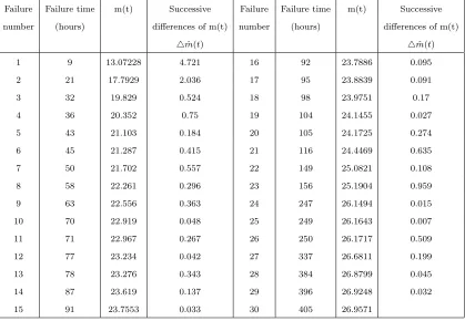
Estimated values of m(t) at the given failure timest1, t2, ..tn along with the successive differences of these
estimates are given in Table 3. The successive differences would indicate the estimated number of failures
between consecutive failure times. The graph through [ti,4mˆ(ti)] i=1,2,..,n-1 along with three parallel
Fig 1. Control chart based on successive differences of mean value function of DD
3.1. Comparative study.
For comparison, we take Exponential model, the most frequently used model in reliability studies. The
cumulative distribution function of Exponential distribution(ED)is
F(x) = 1−e−bx, x >0, b >0. (3.8)
The NHPP withθF(x) as the mean value function for our present study is
m(x) =θ[1−e−bx], x >0, θ >0, b >0. (3.9)
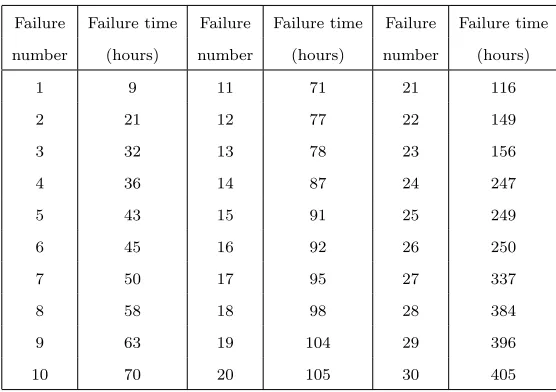
Table 1. Failure time data
Failure Failure time Failure Failure time Failure Failure time number (hours) number (hours) number (hours)
1 9 11 71 21 116
2 21 12 77 22 149
3 32 13 78 23 156
4 36 14 87 24 247
5 43 15 91 25 249
6 45 16 92 26 250
7 50 17 95 27 337
8 58 18 98 28 384
9 63 19 104 29 396
Table 2. Parameter estimates of Dagum distribution and their control limits
Dagum model
a b p θˆ m(tL) m(tC) m(tU)
0.6 0.5 5 29.47 0.0398 14.7349 29.4302
Table 3. Successive differences based on the mean value function of DD
Failure Failure time m(t) Successive Failure Failure time m(t) Successive number (hours) differences of m(t) number (hours) differences of m(t)
4mˆ(t) 4mˆ(t)
1 9 13.07228 4.721 16 92 23.7886 0.095
2 21 17.7929 2.036 17 95 23.8839 0.091
3 32 19.829 0.524 18 98 23.9751 0.17
4 36 20.352 0.75 19 104 24.1455 0.027
5 43 21.103 0.184 20 105 24.1725 0.274
6 45 21.287 0.415 21 116 24.4469 0.635
7 50 21.702 0.557 22 149 25.0821 0.108
8 58 22.261 0.296 23 156 25.1904 0.959
9 63 22.556 0.363 24 247 26.1494 0.015
10 70 22.919 0.048 25 249 26.1643 0.007
11 71 22.967 0.267 26 250 26.1717 0.509
12 77 23.234 0.042 27 337 26.6811 0.199
13 78 23.276 0.343 28 384 26.8799 0.045
14 87 23.619 0.137 29 396 26.9248 0.032
15 91 23.7553 0.033 30 405 26.9571
Table 4. Parameter estimates of Exponential model and their control limits
Exponential model
b θˆ m(tL) m(tC) m(tU)
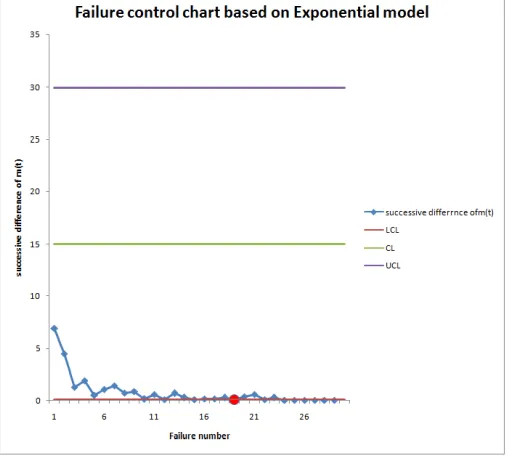
Table 5. Successive differences based on the mean value function of ED
Failure Failure time m(t) Successive Failure Failure time m(t) Successive number (hours) differences of m(t) number (hours) differences of m(t)
4mˆ(t) 4mˆ(t)
1 9 7.09865 6.924 16 92 28.1014 0.163
2 21 14.0223 4.491 17 95 28.2648 0.149
3 32 18.5133 1.299 18 98 28.4142 0.261
4 36 19.8122 1.93 19 104 28.6754 0.039
5 43 21.742 0.481 20 105 28.7146 0.361
6 45 22.2229 1.083 21 116 29.0759 0.581
7 50 23.7345 1.428 22 149 29.6567 0.065
8 58 24.7345 0.733 23 156 29.7218 0.26
9 63 25.468 0.858 24 247 29.982 0.001
10 70 26.3264 0.109 25 249 29.2831 0.0005
11 71 26.435 0.587 26 250 29.9836 0.0153
12 77 27.0223 0.088 27 337 29.9989 0.00009
13 78 27.1103 0.684 28 384 29.9999 0.000009
14 87 27.7941 0.249 29 396 30 0.000005
15 91 28.0436 0.058 30 405 30
4. Monitoring the production process based on mean value function using order statistics
Letx1, x2, .., xn be a random sample of sizen representingn inter failure times of a product governed by
the probability model of a continuous random variable X. Let F(x) be the cumulative distribution function
of X. These inter failure times can be used for assessing the failure phenomenon with respect to two limits of
reference called control limits with a pre specified coverage probability. Thus the time control chart plotted
for inter failure times would indicate alarms, advantages and stable failure process. If r is a natural number
(<n), the summations
r P
i=1 Xi,
2r P
i=r+1 Xi,
3r P
i=2r+1
Xietc represent the lapse of time consecutively between every
rth failure. A control chart for times between every rth failure would throw light on the out of control
signals than that of inter failure times. Xieet al(2002) [4] named such a control chart as tr-control chart
and developed control limits using the sampling distribution of
r P
i=1
Xi. They have taken the example of
exponential distribution and used the theory that the sum of exponential variates is a gamma variate to get
the percentiles oftr-control chart with the help of cumulative summations. If the inter failure times are not
exponentials, the control limits oftr-chart of Xieet al(2002) [4] can not be used.
Overcoming this drawback we suggest the following alternative approach to get control limits of tr-chart
for Dagum distribution. If (X1, X2, .., Xr); (Xr+1, Xr+2, .., X2r); (X2r+1, X2r+2, .., X3r); etc are regarded as
independent samples of size r each, i.i.d random variables having F(x) as their common model. Y1 =X1 ,
Y2= 2
P
i=1
Xi,Y3= 3
P
i=1
Xi, ...,Yr= r P
i=1
Xi becomes an ordered sample of sizerrepresenting the time to first
failure, time to second failure, time to third failure,..., time to rth failure respectively. Thus, thet r-chart
is the control chart with Yr as the points on it representing the time to everyrthfailure. Therefore, when
ris fixed, the percentiles of highest order statistics in a sample of sizer would serve the purpose of control
limits for thetr-chart.
Let F(x) be the cumulative distribution function of a continuous positive valued random variable. If the
random variable is taken as representing inter failure time of a device, a control chart of such data with order
statistics would be based on 0.9973 probability limits of the times between failure random variable say t.
These limits and the central line are respectively the solutions of the following equations taking equi-tailed
probabilities.
[F(t)]r= 0.00135 (4.1)
[F(t)]r= 0.5 (4.2)
[F(t)]r= 0.99865 (4.3)
LettU,tC andtL be respectively the solutions of equations (3.1), (3.2) and (3.3) in the standard form
tL=F−1(0.00135
1
tC=F−1(0.5
1
r) (4.5)
tU =F−1(0.99865
1
r) (4.6)
The NHPP withθ.F(x) as the mean value function for our present study is
m(x) =θ
1 +x b
−a−p
, θ >0, a >0, b >0, p >0. (4.7)
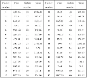
The above model is illustrated for the example of 60 failure times considered by Xieet al(2002) [4]. For
a ready reference the data is produced in table 6.
Table 6. Failure time data of the components
Failure Time Failure Time Failure Time Failure Time
number number number number
1 1065.55 16 2932.96 31 35.85 46 239.66
2 535.8 17 987.67 32 362.8 47 93.78
3 540.53 18 1816.18 33 357.85 48 680.45
4 716.2 19 117.21 34 334.48 49 4.83
5 2525.43 20 190.65 35 80.13 50 102.91
6 1264.18 21 943.99 36 1939.0 51 479.05
7 479.44 22 1084.48 37 77.88 52 156.67
8 1783.22 23 2306.54 38 4.03 53 1286.24
9 473.67 24 6.56 39 98.67 54 443.97
10 2265.42 25 3111.51 40 17.19 55 360.03
11 2191.75 26 283.86 41 289.79 56 414.66
12 1097.26 27 659.39 42 63.99 57 128.9
13 597.59 28 683.48 43 2.46 58 36.1
14 971.16 29 36.14 44 697.68 59 197.31
Table 7. Accumulation failure time for every three failures
Observation Accumulation Observation Accumulation of 3 failures of 3 failures
1 2141.88 11 756.5
2 4505.81 12 2353.61
3 2736.33 13 180.58
4 5554.43 14 370.97
5 4726.04 15 1867.47
6 5736.81 16 1013.89
7 1251.85 17 586.79
8 3397.58 18 1886.88
9 4054.76 19 903.59
10 1473.78 20 651.53
Table 8. Parameter estimates of Dagum distribution and their control limits
Dagum model
a b p θˆ m(tL) m(tC) m(tU)
0.8 0.1 0.5 20.9884 0.000015 4.7555 20.9278
Table 9. Mean value function for accumulated failure times of DD
Observation Accumulation m(t) Observation Accumulation m(t)
of 3 failures of 3 failures
1 2141.88 20.881 11 756.5 20.741
2 4505.81 20.929 12 2353.61 20.888
3 2736.33 20.899 13 180.58 20.222
4 5554.43 20.938 14 370.97 20.554
5 4726.04 20.931 15 1867.47 20.868
6 5736.81 20.939 16 1013.89 20.793
7 1251.85 20.823 17 586.79 20.686
8 3397.58 20.913 18 1886.88 20.869
9 4054.76 20.923 19 903.59 20.774
Fig 3. Control chart based on accumulated failures of mean value function of DD
4.1. Comparative study based on accumulated failure times.
We compare our model under study with the exponential model using the data set given in table 6 and the
results are as follows:
Table 10. Parameter estimates of Exponential model and their control limits
Exponential model
b θˆ m(tL) m(tC) m(tU)
0.02 20.00004 1.5023 13.0130 19.8830
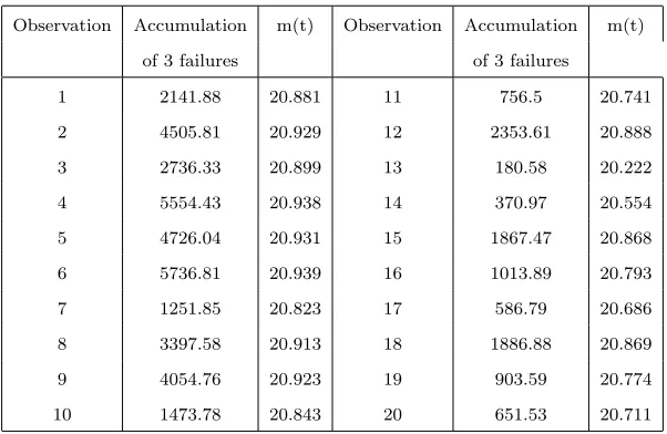
Table 11. Mean value function for accumulated failure times of ED
Observation Accumulation m(t) Observation Accumulation m(t)
of 3 failures of 3 failures
1 2141.88 20.00004 11 756.5 20.00004
2 4505.81 20.00004 12 2353.61 20.00004
3 2736.33 20.00004 13 180.58 19.45987
4 5554.43 20.00004 14 370.97 19.98805
5 4726.04 20.00004 15 1867.47 20.00004
6 5736.81 20.00004 16 1013.89 20.00004
7 1251.85 20.00004 17 586.79 19.99988
8 3397.58 20.00004 18 1886.88 20.00004
9 4054.76 20.00004 19 903.59 20.00004
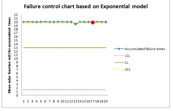
Fig 4. Control chart based on accumulated failures of mean value function of ED
5. Summary & Conclusions
In Figure 1, the first out of control situation is noticed at the 15thfailure with the corresponding successive
difference ofm(t) falling below LCL and hence a preferable out-of-control signal for the product. Where as
in Figure 2, it is noticed at 19thfailure. The earlier the failure, one can alert the process and assignable cause
for this is to be investigated and can be promoted. There are many charts which use statistical techniques.
It is important to use the best chart for the given data, situation and need. In the first part of the paper,
the control chart for estimated number of failures in successive failure time intervals against the serial order
of the failure interval is developed with the associated control lines and central line at same serial point on
that of Kim(2013) [2].
Similarly for the control limits based on the accumulated failure times also shows that Dagum distribution
is better model when compared with that of the exponential model used by Xieet al(2002) [4]. From the
figure 3 and 4 we can observe that 2nd and 19th accumulated failure time is out of the limits respectively.
The earlier the failure group, one need not to wait till the last group failure occurs.
References
[1] Chan, L.Y., Xie, M. and Goh, T.N. Cumulative quality control charts for monitoring production process, Int. J. Product. Res., 38(2)( 2000), 397–408.
[2] Kim, H.C. Assessing software reliability based on NHPP using SPC, Int. J. Softw. Eng. Appl., 7(6)(2013), 61–70. [3] Pham, H. and Zhang, X. Non homogeneous poisson process software reliability and cost models with testing coverage, Eur.
J. Oper. Res., (145)(2003), 443–454.