A Novel Shade to Obtain an Optimal Solution to a Fully Fuzzy Linear Programming Problem

(1)

IJSRR, 7(3) July – Sep., 2018 Page 2086

Review article

Available online www.ijsrr.org

ISSN: 2279–0543

International Journal of Scientific Research and Reviews

A Novel Shade to Obtain an Optimal Solution to a Fully Fuzzy Linear

Programming Problem

Sundari M. Shanmuga

Department of Mathematics,Faculty of Science and Humanities,

SRM Institute of Science and Technology, Kattankulathur, Chennai - 603203, India.

Email: [email protected]

ABSTRACT

A different shade provided in this paper, is to find an optimal solution of a fully fuzzy linear programming problem. A different ranking method is provided for solving linear programming problem in a fuzzy uncertain environment. The proposed method is easy to understand and to apply for fully fuzzy linear programming in real life and flexible as compared to the existing one. Advantages of the proposed method over existing methods are discussed and to illustrate this method, a numerical example is solved and results are also discussed.

KEYWORDS:

Fuzzy sets, Fuzzy number, Trapezoidal Fuzzy number, Fuzzy arithmetic, Fuzzy Ranking.

*Corresponding author

Dr. M. Shanmuga Sundari

Department of Mathematics,

Faculty of Science and Humanities,

SRM Institute of Science and Technology,

Kattankulathur, Chennai - 603203, India.

(2)

1. INTRODUCTION

A typical mathematical program consists of a single objective function, representing either

profits to be maximized or costs to be minimized and a set of constraints that circumscribe the

decision variables. Decision making under fuzzy environment was first proposed by Bellman and

Zadeh 1 The idea was adopted by several authors for solving fuzzy linear programming problems.

Zimmermann2 proposed an application of fuzzy optimization techniques to linear programming

problem with single and multi-objective functions Rommel fanger et al3. Fang and Hu4, Maleki et

al5, Maleki6 and Khan et al7 are studies where the objective functions, the decision variables, the

technical coefficients and the constraints are fuzzy numbers respectively. All these studies

considered fuzzy linear programming problems in which some of the parameters are crisps. Nasseri

et al8 and Amiri and Nasseri9 are some examples utilizing ranking function method for solving

linear programming problems without converting the problem to its crisp equivalent. The FLP

problem is said to be a fully fuzzy linear programming (FFLP) problem if all parameters and

variables are considered as fuzzy numbers. Recently, two methods have been introduced to solve the

FFLP problems by Lotfi et al10 and Kumar et al11. In the first method10 the parameters of FFLP

problem have been approximated to the nearest symmetric triangular fuzzy numbers. After that, a

fuzzy optimal approximation solution has been achieved by solving a multi objective linear

programming (MOLP) problem. As a resulting the optimal solution of FFLP is not exact. So, it is not

reliable solution for decision maker. In the second method11 an exact optimal solution is achieved

using a linear ranking function. In this method, by the above ranking has been used to convert the

fuzzy objective function to the crisp objective function. By this method, fuzziness of objective

function has been neglected by the linear ranking function so by this method the originality

of the problem will get changed . Now Our ultimate aim is to solve the given FFLPP without

sacrificing the originality of the problem that means without converting them to a classical one. So in

this paper we provide a new version of solving FFLPP. In general, most of the existing methods

provide only crisp solutions for the fully fuzzy linear programming problem. In this paper we

propose a simple method, for the solution of fully fuzzy linear programming problem without

converting them in to classical fully fuzzy linear programming problem. The rest of this paper is

organized as:In section 2, we recall the basic concepts and the results of trapezoidal fuzzy numbers

and their arithmetic operations. In section 3, we define fully fuzzy linear programming problem and

prove some of the important theorems, related results and also fuzzy version simplex algorithm is

(3)

IJSRR, 7(3) July – Sep., 2018 Page 2088 for the fully fuzzy linear programming problem without converting them to classical linear

programming problem and the results obtained are discussed.

2 PRELIMINARIES

The aim of this section is to present some notations, notions and results which are of useful in

our further consideration.

2.1 Fuzzy number

A fuzzy set Ã defined on the set of feal numbers R is said to be a fuzzy number if its

membership function : 0 ,1

A R

  _ _ has the following characteristics

(i) Ã is normal. It means that there exists an xR such that   1

A

x  

(ii)A is convex.

 







   



 

1 2

1 2 1 2

A A A

It m e a n s th a t fo r e v e ry x , x R ,

x 1 x m in x , x , 0 ,1



_      _ _  

(iii) _A is upper semi continous.

(iv)supp (A) is bounded in R.

2.2 Trapezoidal Fuzzy Number

A trapezoidal fuzzy number Ã is denoted as Ã = a , a , a , a ₁ ₂ ₃ ₄and is defined by the

membership

function

1

1 2

2 1

A

4

4 3

2 3

3

o t h e r w i s e

x - a

, a x a a - a

1, a x a ( x )

a - x

, a x a a - a

0 ,

        

 

 

 



We use F(R) to denote the set of all trapezoidal fuzzy numbers. Also if m ( A ) represents the

mid point, w ( A ) represents the width,   ( a₂ a )₁ represents the left spread and   ( a4 a )3

represents the right spread of the trapezoidal fuzzy number Ã, then the trapezoidal fuzzy number Ã

(4)

2.3 Ranking of trapezoidal fuzzy numbers

Several approaches for the ranking of fuzzy numbers have been proposed in the literature. An

efficient approach for comparing the fuzzy numbers is by the use of a ranking function based on their

graded means. That is, for every : F R  Rwhich maps each trapezoidal fuzzy number into a real

number, where a natural order exists

For every trapezoidal fuzzy number Ã = a , a , a , a ₁ ₂ ₃ ₄

, ranking function : F R  R is

defined by graded mean as

 

2 3

( ) ( )

2 4

a a

A   

   

For any two trapezoidal fuzzy numbers Ã = a , a , a , a ₁ ₂ ₃ ₄ and B  b1,b2,b3,b4

 _{we have the}

following comparison

 

i A B i f a n d o n ly i f A B

i i A B i f a n d o n ly i f A B

i i i A B i f a n d o n ly i f A B

i v A B 0 i f a n d o n ly i f A B 0

 

   

     

 _   _ 

 _   _ 

   

    

A trapezoidal fuzzy number A a1,a2,a3,a4 F R



is said to be positive if  A 0

Also 0 

 

0

  

A if A

and A 0 if A 0

 _   _

If  A   B then the trapezoidal fuzzy numbers A a n d B  are said to be equivalent and it is denoted

by A B .

2.4 Arithmetic operations on trapezoidal fuzzy numbers

For any two arbitrary trapezoidal fuzzy numbers Ã a , a , a , a ₁ ₂ ₃ ₄( m ( Ã ), w ( Ã ), , )

, the

arithmetic operations are defined as follows:

(i). Addition: A B ( m ( A ) m ( B ), m a x w ( A ) , w ( B ) , m a x (   ₁,₂), m a x (₁,₂) )

(ii). Subtraction: AB ( m ( A )m ( B ), m inw ( A ) , w ( B ) , m in ( 1,2), m in ( 1, 2) )

      ₎

(iii). Multiplication: A B  ( m ( A ) m ( B ), m a x  w ( A ) , w ( B ) , m a x (   ₁,₂), m a x (₁,₂) )

(5)

3 MAIN RESULTS

3.1 General form of Fully Fuzzy Linear Programming

Optimize (m a x o r m in ) z( c x11c2x2c3x3...cnxn)

subject to the following constraints,

 

1 1 1 1 2 2 1 3 3 1 n n 1

2 1 1 2 2 2 2 3 3 2 n n 2

3 1 1 3 2 2 3 3 3 3 n n 3

m 1 1 m 2 2 m 3 3 m n n m

a x a x a x . . . a x , , b

. . . . . . . . . . . . . .

a x a x a x . . . a x , , b

      



      



       



       



       

...(1)

where

(i). x , x1 2 , x3 ... , xn are fuzzy decision variables.

(ii). c , c , c , ... c1 2 3 n are called fuzzy cost or fuzzy profit coefficients.

(iii). ai j ; i 1, 2 , 3 ....m , j 1, 2 , 3 ...n are called structural fuzzy

coefficients.

(iv). b , b , b , . . . , b1 2 3 m

   

represent fuzzy requirements or fuzzy availability of

m constraints.

(v). The expression



  , ,



_{means that each constraint may take}

only one of the three possible forms.

(vi). The restrictions x j  0 simply implies that the x j must be non

negative.

That is (m a x o r m in ) zc x

(6)

1 X n

1 2 3 n

n X 1

1 2 3 n

m X 1

1 2 3 m

1 1 1 2 1 n

2 1 2 2 2 n

i j m x n

m 1 m 2

w h e r e c c , c , c , . . . c F ( R )

x x , x , x . . . , x F ( R ) ; b b , b , b , . . . , b F ( R ) a n d

a a . . . a a a . . . a A ( a ) . . . .

. . . . a a . . . a

 

 

    

  

 _

  

m x n

m n

( F ( R ) )

 

 

  

 

 

Definition 3.1. The standard form of fully fuzzy linear programming

problem is defined as (m a x o r m in ) zc x

subject to A x   b a n d x  0

Definition 3.2. Any n X 1

1 2 3 n

xx , x  , x ... , x  F ( R ) where

each xi F ( R ) which satisfies the constraints and non-negativity

restrictions of (1) is said to be a fuzzy feasible solution to (1).

Definition 3.3. Let S be the set of all fuzzy feasible solutions of (1).

A fuzzy feasible solution x0S is said to be a fuzzy optimum solution

to (1) if c x0c x fo r a ll x  S w h e re c  c , c , c , ... c1 2 3 n and

1 1 2 2 3 3 n n c x  c x  c x c x  ...c x .

Definition 3.4. Let xx , x1 2, x3 ... , xn. Suppose x solves A xb



  _. _If _all

j j j j j

x  ( m ( x ), w ( x ),   , )  0 for all j=1,2,...,n, then x is said

to be a fuzzy basic solution. If not, x has some non-zero components,

say x , x1 2, x3 ... , xk ,1k n . Then A xb



  _{can be written as:}

1 1 2 2 3 3 k k

1 1 2 2 3 3 k k k 1 k 1 k 2 k 2 n n

j

a x a x a x ... a x b

a x a x a x ... a x a x a x .... a x b

w h e r e x 0 f o r a ll j k 1, k 2 , ...n

   

    

         

   

       

             

 

If the columns a , a , a , ....a1 2 3 k corresponding to these non-zero components x , x1 2, x3 ... , xk are linearly

independent, then x is said to be a fuzzy basic solution.

Theorem 3.1. Let 1

B

x  B b be a fuzzy basic feasible solution of

(2). If for any column a_j in A w h ic h is n o t in B  , the condition

 

(7)

one of the columns in B by a_j

. Proof

Suppose that





1 2 3

, , ...

m

B B B B B

x_  x_ x_ x_ x_ be a fuzzy basic feasible solution with k positive

components such that

B

B x   b or

1

B

x  B b

   



, , ,



0 1, 2 , ... 0 1, 2 , ...

i i i

i

i i

B B B

B

w h e r e x m x w x f o r i k

a n d x f o r i k k m

 

 

   

  



   

 

Now equation B x _B  b becomes

1 1

0 ...(3 )

i

k m

B

i i k

x b b b

  

 



 



  

Then for any column a_j of A which is not in B , we write

m

j i j i 1 j 1 2 j 2 r j r m j m j i 1

a y b y b y b ... y b ... y b y B



             



We know that if the basis vector br

 _{for which}

r j

y  0 is replaced by

j

b of A then the new set of vectors  

1 2 3 r 1 j r 1 m

b , b , b , ..., b    _ , b , b  _ , ...b still form a basis. Now for

r j

y  0_and_{r ≤ k}_{, we can write}

1 ,

1 1

m

j i j

i i r

r j r j

k m

j i j i j

i i k

r j r j r j

a y

b b

y y

a y y

b b

y y y

 

  

 

  





 



 

(8)

1 , 1

1 , 1 1 1

1 , 1 . 1

0

i r

r r r

i

k m

i r

B B

i i r i k

k k m m

j i j i j

i i i i

B B

i i r r j i r j i k r j i k

k k m

B B B

i j i j i i j

B

i i r r j r j i i r r j i k

x b x b b b

a y y

x b x b b b b

y y y

x x x

x b a y b y

y y y

                        _   _                                                1

1 , 1 1

1 ,

0

S i n c e 0 ; f o r i = k + 1 ; k + 2 , . . . m , w e h a v e

r r r

i i r i m i i i k

k m m

B B B

i j i j i j

B

i i r r j r j i k r j i k

B k

B

i j i

B

i i r r j

b b b

x x x

x y b a y b

y y y

x

x y b

y                  _  _   _  _                                              

 ₁ ₁

1 ,

ˆ ˆ _{. . . ( 4 )}

ˆ _; r r i r r i i r r i i m m B B

j B i j

i k i k

r j r j

m

B B

i j i j

B

i i r r j r j

m

i j

B B

i i r

B i j

B B

r j

x x

a x y b

y y

x x

x y b a b

y y

x b x a b

x

w h e r e x x y

y            _  _                                                     ˆ r r B B r j i r x x y      

which gives a new fuzzy basic solution to A x b . We shall show that this new fuzzy basic solution

is also feasible. This requires that

0 ;

0

0 m i n ; 0

m , , , m , ,

r i r i r i r i i r r B i j B r j B r j B B

r j i j

B B

r j i j

B B

B B _r _r

r j r j r j r j i j i j

x

x y i r

y x

y

x x

S e l e c t y s u c h t h a t y

y y x x y y x x x x w w

y y y y y y

         _ _                _ _ _ _  _ _ _ _                                        _ _ ,

m , , , m , , , 0

m m , m i n ,

i i r r

i r i

i i

i j i j

B B i i B B r r

i j i j i j i j r j r j r j r j

B B B B

i j r j i j

y y

x x x x

w w

y y y y y y y y

x x x x

w w

y y y

                             _ _ _ _   _ _ _ _                                                       _   _      

, m i n , , m i n , 0

0

r

i r

i r i r

r j i j r j i j r j

B B

i j r j

y y y y y

x x y y               _ _ _ _ _ _ _ _   _ _ _ _ _ _                 

Hence the new fuzzy basic solution is a fuzzy basic feasible solution.

(9)

IJSRR, 7(3) July – Sep., 2018 Page 2094 problem is convex.

Proof

Let SF₀

 _{denote the set of optimal solution}

. If SF₀

 _{is empty or singleton , then it is convex.}

Let SF₀

 _{contain more than one solution say}

0

1 2 F

x , x  S

Then c x1c x2 m a x z

Consider convex combination of x , x1 2as

 

0

0 1 2

1 2

0 F

W x 1 x

c W c x 1 x

c x 1 c x

m a x z 1 m a x z m a x z

W S

              

     

 

 _ _



   

 

 

  

HenceSF₀

 _{is convex.}

3.3 Fuzzy version of simplex algorithm

Step 1: Formulate the Fuzzy linear programming problem for the given data.

Step 2:Express the FFLP in the standard form by adding slack variables in the left hand side of less than or equal to constraint as well as

to the objective function.

Optimize ( m a x o r m in ) z( c x1 1c2x2c3x3...cnxn) 0 s10 s20 s3....0 sm

   

       

    

subject to the fuzzy linear constraints,

1 1 1 1 2 2 1 3 3 1 n n 1 1

2 1 1 2 2 2 2 3 3 2 n n 2 2

3 1 1 3 2 2 3 3 3 3 n n 3 3

m 1 1 m 2 2 m 3 3 m n n m m

1 2

a x a x a x . . . a x s b

. . . . . . . . . . . . . .

a x a x a x . . . a x s b

a n d x , x , x

     



       



        



        



        

  

3 . . . , x n , s1, s2, . . . .sm  0



  



Where s , s , ...s1 2 mare slack variables which have been assigned zero

fuzzy coefficient in the objective function.

(10)

IJSRR, 7(3) July – Sep., 2018 Page 2095 Before the initial simplex tableau can be set up obtain the initial

Feasible solution By setting x1 x2  x3... xn 0



    _{such that in}

the constraint set, we get

1 1 2 2 3 3 m m

s  b , s  b , s  b ..., s  b

   

Step 4:Set up the initial tableau

Step 5:Test for optimality

If all the elements in the cjzj are negative or equal to zero then the

current solution is optimal.If there exists some positive fuzzy number

,the current solution can be improved by removing one basic variable

from the basis and replacing it by some non basic one.

Step 6:Revising simplex tableau At each iteration ,the simplex method moves from the current basic feasible solution to a better basic feasible

solution.

(i)Determine the entering variable.

(ii) Determine the leaving variable.

(iii)Identify the pivotal number.

Step 7: construct a new simplex tableau. (i) Compute new values for the pivotal row.

(ii) compute fresh values of the remaining rows as

 

N e w r o w n u m b e r  O ld r o w n u m b e r e le m e n t in th e p iv o t r o we le m e n t in th e p iv o t r o w p iv o t n u m b e r

Step 8:Test the optimality

Step 9:If any of the numbers in cjzjrow are positive, repeat the

entire step 5 and 6 again.This process is repeated until an optimal

solution has been obtained.

4 Numerical Examples

The following examples are taken from the paper solving fully fuzzy linear

programming problem with inequality constraints by Amit Kumar,

Jagdeep Kaur [3].

Example 4.1. Solve m a x z1, 3, 5, 7x1 2 , 4 , 6 , 8x2 Subject to the constraints,

     

1 2

0 , 2 , 4 , 5 1, 2 , 3 , 4 1, 1 0 , 2 7 , 4 8 2 , 4 , 5 , 6 2 , 4 , 6 , 8 4 , 2 0 , 4 5 , 8 0

x x

 

 

(11)

Solution

First we convert the trapezoidal fuzzy number Ã a , a , a , a ₁ ₂ ₃ ₄( m ( Ã ), w ( Ã ), , )

  1   2

m a x z 4 ,1, 2 , 2 x  5,1, 2 , 2 x

Subject to the constraints,

     

1 2

3 , 1, 2 , 1 2 .5 , .5 , 1, 1 1 8 .5 , 8 .5 , 9 , 2 1 4 .5 , .5 , 2 , 1 5 , 1, 2 , 2 3 2 .5 , 1 2 .5 , 1 6 , 3 5

x x

 

 

Standard form is

  1   2   1   2

m a xz 4 ,1, 2 , 2 x  5,1, 2 , 2 x  0 , 0 , 0 , 0 s  0 , 0 , 0 , 0 s

       

1 2 1

1 2 2

3 , 1, 2 , 1 2 . 5 , . 5 , 1, 1 1, 0 , 0 , 0 1 8 . 5 , 8 . 5 , 9 , 2 1 4 . 5 , . 5 , 2 , 1 5 , 1, 2 , 2 1, 0 , 0 , 0 3 2 . 5 , 1 2 . 5 , 1 6 , 3 5

x x s

  

  

The basic solution is

 

1

2

1 8 .5 , 8 .5 , 9 , 2 1 3 2 .5 , 1 2 .5 , 1 6 , 3 5

s

   

Table 1: Initial table

j

c 4 ,1, 2 , 2 5 ,1, 2 , 2 0 , 0 , 0 , 0 0 , 0 , 0 , 0

B

c B xB x1 x2 s1 s2 Row

minimum

0 , 0 , 0 , 0 s1 1 8 .5, 8 .5, 9 , 2 1 3,1, 2 ,1 2 .5, .5,1,1 1, 0 , 0 , 0 0 , 0 , 0 , 0 7 .4 , .5,1,1

0 , 0 , 0 , 0 s2 3 2 .5,1 2 .5,1 6 , 3 5 4 .5, .5, 2 ,1 5 ,1, 2 , 2 0 , 0 , 0 , 0 1, 0 , 0 , 0 6 .5,1, 2 , 2

j

z _{0 ,1 2 .5,1 6 , 3 5} _{0 ,1, 2 ,1} _{0 ,1, 2 , 2} _{0 , 0 , 0 , 0} _{0 , 0 , 0 , 0}

j j

c  z _{4 ,1, 2 ,1} _{5 ,1, 2 , 2} _{0 , 0 , 0 , 0} _{0 , 0 , 0 , 0}

2

x is entering ,s₂ is leaving

(12)

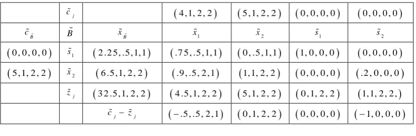
IJSRR, 7(3) July – Sep., 2018 Page 2097 Table 2: First iteration table

j

c _{4 ,1, 2 , 2} _{5 ,1, 2 , 2} _{0 , 0 , 0 , 0} _{0 , 0 , 0 , 0}

B

c B x_B x1 x2 s1 s2

0 , 0 , 0 , 0 s1 2 .2 5, .5,1,1 .7 5 , .5 ,1,1 0 , .5 ,1,1 1, 0 , 0 , 0 0 , 0 , 0 , 0 5 ,1, 2 , 2 x2 6 .5,1, 2 , 2 .9 , .5, 2 ,1 1,1, 2 , 2 0 , 0 , 0 , 0 .2 , 0 , 0 , 0

j

z _{3 2 .5,1, 2 , 2} _{4 .5,1, 2 , 2} _{5 ,1, 2 , 2} _{0 ,1, 2 , 2} _{1,1, 2 , 2 ,}

j j

c  z __{.5, .5, 2 ,1} _{0 ,1, 2 , 2} _{0 , 0 , 0 , 0} __{1, 0 , 0 , 0}

All c_j z_j  0

The current solution is optimal.

 

1

2

3 2 .5 , 1, 2 , 2

2 9 .5 , 3 1 .5 , 3 3 .5 , 3 5 .5 0 , 0 , 0 , 0

6 .5 , 1, 2 , 2 3 .5 , 5 .5 , 7 .5 , 9 .5

z

x

  

  

 

These results are sharper than the results obtained by the existing method.

Example 4.2

Solve m a xz 0 ,1, 2 , 3x₁ 2 , 3, 4 , 5x₂

     

1 2

1, 2 , 3 , 4 3 , 2 , 5 , 1 0 1 5 , 1 0 , 3 2 , 7 4 2 , 3 , 5 , 6 4 , 5 , 7 , 8 8 , 2 1, 4 8 , 7 6 0 , 1, 2 , 3 2 , 4 , 6 , 8 2 , 1 4 , 3 2 , 5 8

x x

   

   

 

 

Solution

First we convert the trapezoidal fuzzy number Ã a , a , a , a ₁ ₂ ₃ ₄( m ( Ã ), w ( Ã ), , )

  1   2

m a x z 1 .5, .5,1,1 x  3 .5, .5,1,1 x

     

1 2

2 .5 , .5 , 1, 1 3 .5 , 1 .5 , 5 , 5 2 1, 1 1, 2 5 , 4 2 4 , 1, 5 , 1 6 , 1, 1, 1 3 4 .5 , 1 3 .5 , 2 9 , 2 8 1 .5 , .5 , 1, 1 5 , 1, 2 , 2 2 3 , 9 , 1 2 , 2 6

x x

 

 

 

 

(13)

       

   

1 2 1 2

1 2

m a x 1 .5 , .5 .1 .1 3 .5 , .5 , 1, 1 0 , 0 , 0 , 0 0 , 0 , 0 , 0 , 0 , 0 , 0 , 0 , 0 , 0

z x x s s

M A M A

   

 

   



       

         

       

1 2 1

1 2 2 1

1 2 2

2 .5 , .5 , 1, 1 3 .5 , 1 .5 , 5 , 5 1, 0 , 0 , 0 2 1, 1 1, 2 5 , 4 2

4 , 1, 5 , 1 6 , 1, 1, 1 1, 0 , 0 , 0 1, 0 , 0 , 0 3 4 .5 , 1 3 .5 , 2 9 , 2 8 1 .5 , .5 , 1, 1 5 , 1, 2 , 2 1, 0 , 0 , 0 2 3 , 9 , 1 2 , 2 6

x x s

x x s A

x x A

  

   

  

  

 

The basic solution is

 

1

2

2 1, 1 1, 2 5 , 4 2 3 4 .5 , 1 3 .5 , 2 9 , 2 8

2 3 , 9 , 1 2 , 2 6

s

A

     

Table 3: Initial table

j

c _{1 .5 , .5 ,1,1} _{3 .5, .5,1,1} _{0 , 0 , 0 , 0}_{0 , 0 , 0 , 0}__M _{, 0 , 0 , 0}__M _{, 0 , 0 , 0}

B

c B x_B x1 x2 s1 s2 A₁ A₂

0 , 0 , 0 , 0 s1 2 1,1 1, 2 5, 4 2 2 .5, .5,1,1 3 .5,1 .5, 5, 5 1, 0 , 0 , 0  

0 , 0 , 0 , 0 0 , 0 , 0 , 0 0 , 0 , 0 , 0

M , 0 , 0 , 0

1

A 3 4 .5,1 3 .5, 2 9 , 2 84 ,1, 5 ,1  6 ,1,1,1 0 , 0 , 0 , 0 1, 0 , 0 , 0 1, 0 , 0 , 0 0 , 0 , 0 , 0

M , 0 , 0 , 0

2

A 2 3, 9 ,1 2 , 2 6 1 .5 , .5 ,1,1 5 ,1, 2 , 2 0 , 0 , 0 , 0 0 , 0 , 0 , 0 0 , 0 , 0 , 0 1, 0 , 0 , 0

j

z 5 7 .5M,1 3 .5 , 2 9 , 4 2 __{5 .5}_M_{,1, 5,1}_ 1 1M,1 .5, 5, 5 0 , 0 , 0 , 0 M, 0 , 0 , 0 M, 0 , 0 , 0 _M, 0 , 0 , 0_

j j

c  z 1 .55 .5M, .5,1,1 3 .51 1M, 1, 2 , 2 0 , 0 , 0 , 0 M, 0 , 0 , 0 0 , 0 , 0 , 0 0 , 0 , 0 , 0

2

x is entering

2

A is leaving

(14)

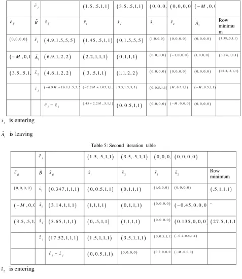
IJSRR, 7(3) July – Sep., 2018 Page 2099 Table 4: First iteration table

j

c _{1 .5 , .5 ,1,1} _{3 .5, .5,1,1} _{0 , 0 , 0 , 0}_{0 , 0 , 0 , 0}__M _{, 0 , 0 , 0}

B

c B xB x1 x2 s1 s2 A₁ Row

minimu m

0 , 0 , 0 , 0

1

s _{4 .9 ,1 .5, 5, 5} _{1 .4 5, .5,1,1} _{0 ,1 .5, 5, 5} 1, 0 , 0 , 0 0 , 0 , 0 , 0 0 , 0 , 0 , 0 3 .3 8, .5,1,1

M , 0 , 0 , 0

1

A 6 .9 ,1, 2 , 2 2 .2 ,1,1,1 0 ,1,1,1 0 , 0 , 0 , 0 1, 0 , 0 , 0 1, 0 , 0 , 0 3 .1 4 ,1,1,1

3 .5, .5,1,1x2 4 .6 ,1, 2 , 2 .3, .5,1,1 1,1, 2 , 2 0 , 0 , 0 , 0 0 , 0 , 0 , 0 0 , 0 , 0 , 0

1 5 .3, .5 ,1,1

j

z 6 .9M 1 6 .1, 1 .5 , 5 , 52 .2M 1 .0 5,1,1,13 .5 ,1 .5 , 5 , 5 0 , 0 .5,1,1 M, 0 .5,1,1 M, 0 .5 ,1,1

j j

c  z .4 52 .2M, .5,1,1  

0 , 0 .5,1,1 0 , 0 , 0 , 0 M, 0 , 0 , 0 0 , 0 , 0 , 0

1

x is entering

1

A is leaving

Table 5: Second iteration table

j

c _{1 .5 , .5 ,1,1} _{3 .5, .5,1,1} _{0 , 0 , 0 , 0}_{0 , 0 , 0 , 0}

B

c B xB x1 x2 s1 s2 Row

minimum

0 , 0 , 0 , 0

1

s _{0 .3 4 7 ,1,1,1} _{0 , 0 .5,1,1} _{0 ,1,1,1} 1, 0 , 0 , 0 0 , 0 , 0 , 0 _{.5 ,1,1,1}

M , 0 , 0 , 0x1 3 .1 4 ,1,1,1 1,1,1,1 0 ,1,1,1 0 , 0 , 0 , 0 0 .4 5, 0 , 0 , 0-

3 .5, .5,1,1x2 3 .6 5,1,1,1 0 , .5 ,1,1 1,1,1,1 0 , 0 , 0 , 0 0 .1 3 5, 0 , 0 , 0 2 7 .5,1,1,1

j

z _{1 7 .5 2 ,1,1,1} _{1 .5 ,1,1,1} _{3 .5 ,1,1,1} 0 , 0 .5,1,1 0 .2 , 0 .5 ,1,1

j j

c  z _{0 , 0 .5,1,1} 0 , 0 , 0 , 0 0 .2 , 0 , 0 , 0 M, 0 , 0 , 0

2

s is entering

1

(15)

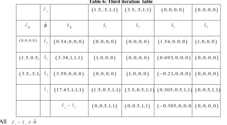
IJSRR, 7(3) July – Sep., 2018 Page 2100 Table 6: Third iteration table

j

c 1 .5 , .5 ,1,1 3 .5, .5,1,1 0 , 0 , 0 , 0 0 , 0 , 0 , 0

B

c B x_B x1 x2 s1 s2

0 , 0 , 0 , 0

2

s 0 .5 4 , 0 , 0 , 0 0 , 0 , 0 , 0 0 , 0 , 0 , 0 1 .5 4 , 0 , 0 , 0 1, 0 , 0 , 0

1 .5, 0 .5,1,1x1 3 .3 8,1,1,1 1, 0 , 0 , 0 0 , 0 , 0 , 0 0 .6 9 3, 0 , 0 , 0 0 , 0 , 0 , 0

3 .5, .5,1,1x2 3 .5 9 , 0 , 0 , 0 0 , 0 , 0 , 0 1, 0 , 0 , 0 0 .2 1, 0 , 0 , 0 0 , 0 , 0 , 0

j

z _{1 7 .6 3,1,1,1} _{1 .5, 0 .5,1,1} _{3 .5, 0 .5,1,1} _{0 .3 0 5, 0 .5,1,1} _{0 , 0 .5,1,1}

j j

c  z _{0 , 0 .5,1,1} _{0 , 0 .5,1,1} __{0 .3 0 5, 0 , 0 , 0} _{0 , 0 , 0 , 0}

All c_j z_j  0

The current solution is optimal.

 

1

2

1 7 .6 3 , 1, 1, 1

1 5 .6 3 , 1 6 .6 3 , 1 8 .6 3 , 1 9 .6 3 3 .3 8 , 1, 1, 1

1 .3 8 , 2 .3 8 , 4 .3 8 , 5 .3 8 3 .5 9 , 0 , 0 , 0

3 .5 9 , 3 .5 9 , 3 .5 9 , 3 .5 9

z

x

   

  



These results are sharper than the results obtained by the existing method.

5 CONCLUSION

Based on the current study it can be concluded that it is better to use proposed version of

solving Fully Fuzzy Linear Programming as it was compared to the existing one. In this paper, a new

algorithm has been suggested to solve the FFLP problem. By simple examples and the obtained

results of proposed algorithm (with Kumar’s method) have been compared and shown the reliability

and applicability of our algorithm

ACKNOWLEDGEMENTS

The authors are grateful to the anonymous referees and the editors for their constructive

(16)

REFERENCES

1. Bellman, R.E and Zadeh, L.A, Decision-making in fuzzy environment,Management sciences,

1970; 17(4): 141- 164

2. Zimmermann H. J, Fuzzy programming and linear programming with several objective

functions, Fuzzy sets and systems, 1978; 1: 45-55.

3. Rommelfanger, H, Hanuscheck, R, and Wolf, J, Linear programming with fuzzy objective,

Fuzzy Sets and Systems, 1989; 29: 31-48.

4. Fang, S. C, and Hu, C. F, Linear programming with fuzzy coefficients in constraint ,Comput

Math Appl, 1999; 37: 63-76,DOI:10.1016/s0898-1221(99)00126-1.

5. Maleki, H. R , Ranking functions and their applications to fuzzy linear programming, Far

East J Math Sci, 2002; 4: 283-301.

6. Maleki, H. R, Tata, M., and Mashinchi, M, Linear programming with fuzzy variables, Fuzzy

sets and systems, 2000; 109: 21-33.

7. Khan, I. U, Ahmad, T, and Maan, N, A two phase approach for solving linear programming

problems by using fuzzy trapezoidal membership functions, International Journal of Basic

and Applied Sciences, 2010; 6: 86-95

8. Nasseri, S. H, Ardil, E, Yazdani, A, and Zaefarian, R , Simplex method for solving linear

programming problems with fuzzy numbers, Proceedings of World Academy of Science,

Engineering and Technology, 2005; 10: 284-288, DOI:10.1.1.192.8585.

9. Amiri, N. M, and Nasseri, S. H, Duality results and a dual simplex method for linear

programming problems with trapezoidal fuzzy variables. Fuzzy Sets and Systems, 2007; 158:

1961-1978, DOI:10.1016/j.fss.2007.05.005.

10. Lotfi, F.H., Allahviranloo, T, Jondabeha, M.A, Alizadeh, L, Solving a fully fuzzy linear

programming using lexicography method and fuzzy approximate solution, Appl. Math.

Model, 2009; 33: 3151-3156, DOI:10.1016/j.apm.2008.10.020.

11. Kumar,A, Kaur,J, Singh,P,A new method for solving fully fuzzy linear programming

problems, Appl. Math. Model, 2011; 35: 817-823, DOI:10.1016/j.apm.2010.07.037.

12. Abbasbandy, S and Hajjari, T, A new approach for ranking of trapezoidal fuzzy numbers,

Computers and Mathematics with Applications,2009; 57:

413419,DOI:10.1016/j.camwa.2008.10.090.

13. Amit Kumar, Jagdeep Kaur, Pushpinder Singh, Solving Fully Fuzzy linear programming

problem with inequality constraints, International Journal of Physical and Mathematical

(17)

14. Kauffmann,A, Gupta, M.M, Introduction to fuzzy Arithmetic:Theory and Applications, Van

Nostrand Reinhold, New York, 1991.

15. Ming Ma, Menahem Friedman, Abraham Kandel, ”A new fuzzy arithmetic” ,Fuzzy sets and