A recommendation-based pricing system for information
goods versioning
Wei-Lun Chang , Assistant Professor
Dept. of Business Administration, Tamkang University, Taiwan
[email protected]
Soe-Tsyr Yuan, Professor
Dept. of Management Information Systems, National Chengchi University, Taiwan
[email protected]
Abstracŵ炼Information goods versioning is an essential and emerging topic of information goods pricing. Myriad researchers have devoted considerable attention to developing and testing methods in terms of versioning. Nevertheless, in addition; there are still certain shortcomings as the challenges to be overcome. This study encompasses the software maintenance concept (mean error rate) to develop a recommendation-based system which maintains the profits automatically with recommendations. The present paper also proposes economic model and algorithm to prove the feasibility with certain contributions: (1) provides an automatic system to maintain the profits, (2) deliberates the recommendations from knowledge base, and (3) offers an appropriate recommendation to versioning strategy.
Index TermŴ 炼Information goods versioning, software maintenance, knowledge base
I. INTRODUCTION
Shapiro and Varian (1998) defined “information goods” broadly as anything that can be digitized and encoded as a stream of bits, and transmitted over information network [5]. Examples of information goods include books, movies, software programs, web pages, song lyrics, television programs, newspaper columns, and o on. Furthermore, these information goods have the property that the fixed-cost of production is high and the marginal cost of reproduction is zero or very low.
The information products may possibly comprise three macro characteristics, which are physical (e.g., indestructibility, transmutability, and reproducibility), spatial/temporal (e.g., enhancement to competition and breaking of local market power), and contingent (e.g., real-time or near real-time)1. McCain (2005) recognized the economic characteristics of information products such as media of transmission (cannot be bought or sold alone), uniqueness, high fixed cost, the incentive problem (little incentive to originate information products due to piracy problem), and intellectual property [4].
1 The Market for Digital Goods: An Overview. http://econ.gsia.cmu.edu/ecommerce/Lecture%202/
Hui and Chau (2002) proposed a classification framework of digital products based on two dimensions, which are product category as well as product characteristic [3]. The dimension of product category identified three categories - tools and utilities (e.g., Adobe Acrobat), content-based digital product (e.g., music, books), and online services (e.g., consulting online). The dimension of product characteristic then recognized three intrinsic characteristics - delivery mode (is the information product downloadable or interactively on a continual basis?), granularity (is it easy to partition the information product?), and trialability (is it easy to try before ordering?).
Furthermore, information product features other characteristics, such as no attrition (the quality would not be distorted over time), easy to copy (without additional cost to make a copy), network externality (the effects of word-of-mouth), easy to change, and experienced good (experience it before purchasing). In short, the information product characteristics and the cost structure (high production cost and low reproduction cost) are profoundly different from the traditional business. The value of information goods also varies among different people and the pricing strategy become volatile.
Due to the unique cost structure and product characteristics 2 of information goods, the possibility to follow traditional pricing strategies becomes unfeasible and the differential pricing strategy is recognized to be crucial [6][7][10][12]. The work of Varian (1997) showed that optimal versioning solution is the best pricing regimes for information goods via examining the total surplus from the economic view [11]. In this category, two orientations of structural elements emerged, which were the internal factors (factors intrinsic to the creation and delivery of a product) and the external factors (factors of no relevance to pro).
When vertically differentiating the market, three versions, in general, is an appropriate versioning policy
when the market segmentation is ambiguous [2]. In addition, there are four practical concerns for a producer: (1) Prepare a product that could be versioned. (2) Differentiate the high end of the market first before segmenting the remaining market. (3) Ensure the versioned products that could be viewed by consumers. (4) Goldilocks pricing3 is recommended for the producer in the absence of any additional information except having three versions.
As for the structural elements of internal factors, the work of Shapiro and Varian (1998) decided an appropriate number of versions in terms of the factors as delay, convenience, comprehensive, manipulation, community, annoyance, speed, data processing, user interface, image resolution, and support [5]. For example, for a product that is of no convenience, slow speed and complicated manipulation, the number and differential level of versions should be short and well-separated.
In the study of Bhargava and Choudhary (2001), several external factors were identified as the other key structural elements to influence the versioning method, which are network effects, advertising revenues, nonlinear utility function, and threat of entry [2]. For instance, high advertising revenues differentiate popular versions from unacceptable versions; high threat of entry requires various versions to segment the market for differentiating the product to win the competition.
The present paper uses design science as the methodology to build an artifact (system) to maintain the profits automatically. Additionally, this work proposes economic model and algorithm to prove the feasibility with certain contributions: (1) provides an automatic system to maintain the profits, (2) deliberates the recommendations from knowledge base, and (3) offers an appropriate recommendation to versioning strategy.
This paper is organized as follows. Section 2 describes the background of the recommendation-based sysetm. Section 3 further provides a economic model with theoretical proofs. Section 4 details the algorithms used in the system. Section 5 then furnishes the simulation model and the performance analysis. Section 6 discusses and summrizes the experiment results. Finally, the conclusion remarks are provided in Section 7.
II. BACKGROUND A. Software Maintenance
Software maintenance is currently an important issue. Previous studies have focused on prevention and elimination of errors in new software [8]. The aim of software maintenance is to produce software that is as
3 The notion of Goldilocks pricing is based on “extremeness
aversion”, which means people tend to choose the mid-range offering rather than traditional two versions of high-end and low-end.
close to error-free as possible. Thus, software maintenance is an ongoing process required to maintain software usability; poorly managed maintenance can result in a steady stream of errors throughout the life of software. In best cases, software failure is only an inconvenience to users [9]. Conversely, in worst cases, software failure can threaten the credibility and viability of an organization.
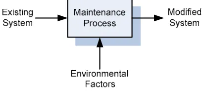
Conceptually, variations in software error rates are likely a function of the software system or factors in the maintenance environment. A maintenance process utilizes the previous system version as the primary input data; however, the process is affected by other factors such as maintainer skills. An existing system can be assessed by measuring reliability to identify the system’s static characteristics that cause high error rates. Most characteristics can be described in terms of software size and complexity. Size, which is measured in thousands of lines of code, is a good predictor of error rates. Complexity is a more sophisticated measure and is used to correct software defects beyond the simple measure of size.
Figure 1 Conceptual model of maintenance process
The factors in a conceptual maintenance model process are insufficient and Y inadequate for illustrating enhanced reliability. Thus, Banker et al. (2002) proposed the following concrete factors that impact error rates: static (size and complexity); dynamic (operational frequency and volatility); and, environmental (maintainer experience and performance requirements) [1]. Error rate is modeled as a stochastic variable and multiplicative function of several explanatory variables pertaining to those systems. In particular, error rate is modeled as a random draw from a lognormal distribution with a mean Lambda (λ), where λ(error rate) = f (static factors, dynamic factors, environmental factors) and f(·) is a multiplicative function4.
For static factors, system size (e.g., thousands of source lines of code) has been employed as a measure of the magnitude of a task performed by a system. The
4 Banker, R. D., Datar, S. M., Kemerer, C. F., and Zweig, D.,
difficulty in measuring software complexity can be solved using numerous measures, such as average module length and average procedure length. Conversely, operational frequency and volatility are factors in the dynamic perspective. Systems that undergo frequent modifications are expected to have high error rates as each modification is an opportunity to generate new errors. Thus, volatility is a characteristic of systems that are subject to ongoing modifications. Additionally, the frequently of software use is directly related to the variety of inputs and amount of errors generated.
Maintainer experience and performance requirements are environmental factors. In terms of maintainer experience, when programmers have little time to maintain systems, relative inexperience will increase the chances of errors slipping being overlooked. Since the effort required to identify errors in existing code typically takes more time than modifying the code, application-specific experience is particularly important to software maintenance. Conversely, the performance requirement identifies systems with particularly rigorous performance requirements (i.e., maintaining requirement efficiencies) as the principal maintenance goal.
In short, this work presents a novel maintenance model for identifying managerial controllable factors that impact software reliability. The experimental results reveal that high error rates can result from (1) frequent modifications, (2) programmers with inadequate experience, and (3) high reliability requirements. Thus, managers can make quality judgments to decrease error rates by implementing a number of key procedures, including enforcing release control, assigning experienced maintenance programmers, and establishing and enforcing complexity metric standards.
B. Mean Error Rate
The error rate is modeled as a random draw from a lognormal distribution with a mean Lambda. The formula is λ= f(static, dynamic, environmental), where f(˙) is a
multiplicative function. Lognormal distribution and
exponential distribution are widely utilized in software reliability literature; both distributions are consistent with the belief that error rates have an early peak and a single long tail.
The parameter value for error rate varies among applications based on the values of structural variables that determine it. The following fixed-effects regression model was estimated as:
parameter residual
the is e and
indicator each
for t coefficien weight
the is ~ where
e ln
6 0
6 5 4 3 2 1 0 β β
β β β β β β
β + + + + + + +
= S C OF V Sa P
ERRORS
The independent variable (ERRORS) is defined as the unselected decision among all versions. That is, the size and complexity are enfolded in the static factors. Size is the number of bundles derived from the version and complexity is the number of different services in the version. Next, the operational frequency and volatility unfolds dynamic factors. Operational frequency is the number of bundles purchased during the previous month (i.e., a user may discard the bundles in the collaborative process and choose the original version). Volatility implies that a version is subject to the number of frequent changes up to present.
Ultimately, environmental factors are decomposed to satisfaction and profit. Satisfaction is from a user’s perspective, whereas profit is considered from a producer’s perspective. Satisfaction indicates is a subjective score assigned by a user, and profit is the average profit for each version.
Furthermore, the system gathers information for each version periodically and estimates the weight coefficients at specific times. Dependent variable ERROR and indicators provide clues for predicting the choice among versions via the significance of weight coefficients. The relative magnitudes of each indicator are determined from a range of values, in which 1 represents extremely high and 0 represents extremely low. Consequently, the coefficient weights assist the system in identifying the difference among indicators and obtain information for further modification of versions.
When identifying new versions, weight coefficients β1–β6 are the significance for each indicator. These
coefficients are normalized to a range of 0–1; thus, differences among the six indicators emerge. The system utilizes a default value as a threshold to determine when to reorganize the version(s). If weight coefficients (β1 andβ2)
exceed the threshold, the system modifies the version(s) depending on the service quality concept (e.g., reduce or increase the number of functions for a service) in the versioning ontology.
Likewise, for dynamic factors, weight coefficients β3
andβ4 reset the time period as a new checkpoint (depends
Table 1 Three factors of error rate
λ= f(static, dynamic, environmental) = ln ERRORS = β0+β1*S +β2*C +β3*OF+β4*V+β5*Sa+β6*P+ε
Static Factors
Size (S) The number of bundles.
Complexity (C) The number of different services in the version.
Dynamic Factors Operational
Frequency (OF)
The number of bundles paid last month.
Volatility (VF) The version is subject to the number of frequent changes up to present.
Environmental Factors Satisfaction (Sa) The subjective score that is assigned by the user.
Profit (P) The average profit for each version.
Ultimately, weight coefficients β5 andβ6 represent the
importance of environmental factors. If the values of these coefficients exceed the threshold, the system re-assembles services based on the service coordination concept in the versioning ontology. Sub-concepts, such as interdependencies (e.g., prerequisite, shared resource, and simultaneity) or goals (e.g., maximize profits or user’s satisfaction), assist the system in enhancing the combination of services in a version. The new version will replace the existing version; this process continues until all versions are verified. Finally, the information for the new version is updated to the GUI module to generate other choices for the user.
This work utilizes the knowledge base to assist version rectification in accordance with the ontology. The system verifies the mean error rate periodically and eliminates/revises versions when needed. The knowledge base is updated automatically when an action is triggered.
III MODEL
Typically, producers determine prices via a versioning paradigm. The goal of versioning is to get customers to sort themselves into groups via different product values; both product design and price are adjusted to affect this sorting (Varian, 1998). A version can include bundled information goods. For example, Microsoft provides enterprise and home editions of Microsoft Office; each version has certain applications.
Supposedly, producers maintain versions based on profits. An un-profitable version can be improved or replaced with a new version. This study then shows that profit is enhanced if and only if the price of the new version is higher than either the original price of a specific version or the average price of all versions.
Thus, we assume that PB is the optimal (equilibrium)
price, PAis the producer acceptable price, PV*is the average
price of all versions, PV’ is the price for a newly revised version, PVis the price of the previously revised version, n
is the number of services in a bundle at an optimal price, r is the average number of services among initial versions, m is
the number of services in a new version, and k is the number of services at the lowest price among all initial versions.
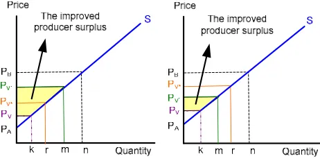
Figure 2 The improved producer surplus of new price
Theorem 1. The profit for a newly revised version is always
enhanced. The enhancement is either wide (when price PV’ is >PV*) or narrow (when price PV’ > PV)5.
Theorem 3 proves that profit is always enhanced for a new version. Lemma 5 confirms that profit at a new price is greater than average price of all previous versions (see left side of Fig.2). Lemma 6 proves the assumption that a new price must be greater than that of the old version (see right side of Fig. 2). The outcomes demonstrate that a service provider should set a new price that is greater than either the average price or previous old price.
Lemma 1. Compared with an average version price PV*,
offering a higher price PV’ improves producer surplus by
(
)
(
' *)
2
1
V V
A
r
m
mP
rP
P
−
+
−
Proof.
First, we assume n>m,r>k and PB > PV’, PV* > PV >
PA. Bundle price should be optimal and always greater than
the price of a newly revised version. The price of either an old version or new version is always low, as bundle price is assumed optimal. In other words, PV* is certainly greater
5 P
V’ is the price for the newly revised version based on
coefficients from the mean error rate equation λ=β0+β1*S +β2*C
than the lowest price PV (i.e., PV* >> PV) according to the
assumption.
If the new price is higher than the average price, then PV’ > PV*. Thus, PV’ - PA > PV* - PA and m > r are true according to PV’ > PV*. Furthermore, producer surplus for
the new price and average price are PSV’ =
2
)
(
P
V'−
P
Am
and PSV* =
2
)
(
P
V*−
P
Ar
.
As this study wants to prove PSV’ > PSV*;
we assume that PSV’ < PSV* (1) Equation (1) can be reduced to
(
P
V'−
P
A)
m
<r
P
P
V A)
(
*−
; however, contradicts PV’ - PA > PV* - PA and m > r. Hence, the original assumption is false; PSV’ > PSV* and the producer surplus is improvedby
(
(
)
' *)
2
1
V V
A
r
m
mP
rP
P
−
+
−
.Lemma 2. Compared with the previous price PV, offering a
higher price PV’ improves producer surplus by
(
)
(
P
Ak
−
m
+
mP
V'−
kP
V)
2
1
;
Proof.
If the new price is higher than the previous price, we presume PV’ > PV. Thus, PV’ - PA > PV - PA and m > k hold. Producer surplus for a new price and previous price are
PSV’ =
2
)
(
P
V'−
P
Am
and PSV ==
2
)
(
P
V−
P
Ak
.
This study wants to prove that PSV’ > PSV, thus, we assume PSV’ < PSV, PSV’ < PSV (2) Equation (2) can be reduced to
(
P
V'−
P
A)
m
<k
P
P
V A)
(
−
, which contradicts PV’ - PA > PV - PA and m > k. Hence, the original assumption is false; PSV’ > PSV and the producer surplus is improved by(
)
(
P
Ak
−
m
+
mP
V'−
kP
V)
2
1
.
Table 2 Price and Producer Surplus
Enhanced Price for a Revised
Version
Average Price among Initial Versions
Previous Price for a Revised Version
Price PV’ PV* PV
Producer Surplus
2
)
(
P
V'−
P
Am
2
)
(
P
V*−
P
Ar
2
)
(
P
V−
P
Ak
Lost profit compared to enhanced price 0
(
)
(
' *)
2
1
V VA
r
m
mP
rP
P
−
+
−
(
P
A(
k
−
m
)
+
mP
V'−
kP
V)
2
1
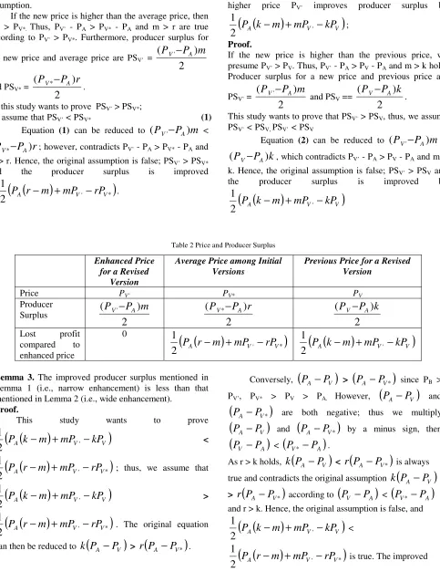
Lemma 3. The improved producer surplus mentioned in
Lemma 1 (i.e., narrow enhancement) is less than that mentioned in Lemma 2 (i.e., wide enhancement).
Proof.
This study wants to prove
(
)
(
P
Ak
−
m
+
mP
V'−
kP
V)
2
1
<(
)
(
' *)
2
1
V VA
r
m
mP
rP
P
−
+
−
; thus, we assume that(
)
(
P
Ak
−
m
+
mP
V'−
kP
V)
2
1
>(
)
(
' *)
2
1
V VA
r
m
mP
rP
P
−
+
−
. The original equationcan then be reduced to
k
(
P
A−
P
V)
>r
(
P
A−
P
V*)
.Conversely,
(
P
A−
P
V)
>(
P
A−
P
V*)
since PB >PV’, PV* > PV > PA. However,
(
P
A−
P
V)
and(
P
A−
P
V*)
are both negative; thus we multiply(
P
A−
P
V)
and(
P
A−
P
V*)
by a minus sign, then(
P
V−
P
A)
<(
P
V*−
P
A)
.As r > k holds,
k
(
P
A−
P
V)
<r
(
P
A−
P
V*)
is alwaystrue and contradicts the original assumption
k
(
P
A−
P
V)
>
r
(
P
A−
P
V*)
according to(
P
V−
P
A)
<(
P
V*−
P
A)
and r > k. Hence, the original assumption is false, and(
)
(
P
Ak
−
m
+
mP
V'−
kP
V)
2
1
<(
)
(
' *)
2
1
V VA
r
m
mP
rP
producer surplus mentioned in Lemma 2 (narrow enhancement) is less than that in Lemma 1 (wide enhancement).
IV ALGORITHM
The error rate (λ) is modeled as a stochastic variable whose mean varies from application system to application system, specifically as a multiplicative function of several explanatory variables pertaining to those systems. (A multiplicative form is used due to the impact of each variable is higher for higher levels of other explanatory variables rather than independent of other variables as in a linear model.)
In particular, the error rate is modeled as a random draw from a lognormal distribution with mean Lambda, the formula represents as λ= f(static, dynamic,
environmental), where f(˙) is a multiplicative function.
The lognormal distribution and the exponential distribution are widely used in the software reliability literature, both being consistent with the intuition that error rates should be distributed with an early peak and a single long tail.
The parameter value of error rate varies from application to application, based on the values of the structural variables which determine it. The following fixed effects regression model was estimated: ln ERRORS = β0+β1*S +β2*C +β3*OF+β4*V+β5*Sa+β6*P+ε, where
β0~β6 is the weight coefficient for each indicator andεis the residual parameter. The independent variable (ERRORS) is defined as the unselected decision among all versions (i.e., unselect or select).
Table 3 The Indicators of Error Rate
λ= f(static, dynamic, environmental) = ln ERRORS = β0+β1*S +β2*C +β3*OF+β4*V+β5*Sa+β6*P+ε
Static Indicators
Size (S) The number of bundles.
Complexity (C) The number of different services in the version. Dynamic Indicators
Operational Frequency (OF) The number of bundles paid last month.
Volatility (VF) The version is subject to the number of frequent changes up to present. Environmental Indicators
Satisfaction (Sa) The subjective score that is assigned by the user. Profit (P) The average profit for each version.
The system gathers the information for each version periodically and initiates the estimation of weight coefficients at a specific time. The dependent variable ERROR provides the clue to predict the discrimination among versions via the significance of weight coefficients. If the error rate is greater than an error threshold, the system terminates the computation. Meanwhile, the system rectifies the version(s) based on versioning ontology and service attribute taxonomy. Subsequently, the new version(s) will be assigned to replace the old one until all versions are verified.
Hence, we come up with an algorithm to detail the process of VR module. In the beginning of the algorithm, the variables are declared in accordance with the definitions. The detailed information (e.g., S, C, OF, V, SA, P) for each version is extracted from price history (PH) and GUI module (Vinfo). Moreover, the system gathers the unselected probability for each version month by month and initiates the estimation of weight coefficients at a specific time period (e.g., 2 months).
Next, the most significant part of the algorithm is the computation of error rate for all versions. If the error rate is greater than a threshold (may be assigned as the mean value based on all existing values of error rate), the system terminates the computation. Meanwhile, the system re-assembles the combination of services in the version (V’)
based on versioning ontology and service attributed taxonomy. The system sets a threshold to determine whether to trigger the revisionary process. If the process is in the progress, the system reassembles the services inside the version and replaces the old one simultaneously. Thus, the non-profit version will be rectified and eliminated in order to provide better versions for choice.
V. EVALUATIONS A. Assumption
Three stereotypes, regular, extroverted, and innovative are employed for three versions. Regular-type consumers make decisions cautiously. Extroverted and innovative people are willing to accept new products and consume a wide range of products. Furthermore, this work assumes the difference among the three versions is not significant. The system has the same foundation to build versions with some dissimilarities for dependent variables, such as number of prototypes (X1), number of services in the version (X2), number of versions to be bought up to the present (X3), number of versions to be modified up to the present (X4), satisfaction (X5), and profit (X6).
innovative-type people likely want to select a version with many services (X2). As the number of services they try increases, the number of prototypes generated increases (X1). The number of prototypes generated has a minor effect on Y. Conversely, people are willing to select a version when they are satisfied with a version (X5).
We also assume the system has a knowledge base for generating versions with increased profitability based on rules derived from economics model. For instance, the prices generated should either be higher than average price or between the lowest and average prices for the three versions of the system based on random combinations. The simulation results are different for various periods, but follow the rules in the knowledge base.
B. Simulation
This study randomizes 20 data with dependent variables (X1 to X6) for each stereotype, and assumes that independent variable Y has is strongly correlated with X2 and X5 (which may have different boundaries for the three consumer stereotypes) and weakly correlated with X1, X3, and X4. The boundary of X1 for each stereotype is 4–7 based on simulation results of ERG need predictions (i.e., a user’s need will converge at 7 steps, and we assume
he/she will assess 4–7 prototypes). The boundaries of X2 for the regular-type consumer is 2–8 (i.e., we assume there are 2–8 services in a version), and the extroverted- and innovative-type consumers assess 2–10 services (i.e., we assume there are 2–10 services in a version).
The boundaries of satisfaction also differ. The regular-type consumer has a range of 5–10 (maximum score is 10) satisfaction score, meaning that consumers decide to select or not select the version cautiously. The extroverted-type consumer has a range for satisfaction of 7–10 and innovative-type consumer has a range of 8–10. These two types of consumers are open-minded to new products; for example, they have a high probability of accepting a high number of service combinations.
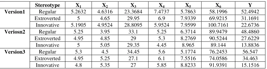
Simulation results indicate that the innovative-type consumer has higher X2 values than the regular-type consumer (e.g., version 1, 4.9524 > 4.6316; version 2, 5.05 > 3.95; version 3, 5.35 > 4.5) (See Table 7-3). Simulation results also suggest that the regular-type consumer has highest average un-selected score (Y) and the innovative-type consumer has lowest average un-selected score for the three versions (e.g., version 1: regular 52.4942 > innovative 22.6736).
Table 4 Average values for dependent and independent variables
Stereotype X1 X2 X3 X4 X5 X6 Y
Version1 Regular 5.2632 4.6316 23.3684 7.4737 5.7863 58.1996 52.4942
Extroverted 5 4.65 29.95 6.9 7.9339 69.9215 31.1691
Innovative 5.1905 4.9524 28.8095 5.9524 7.9599 100.7161 22.6736
Veriosn2 Regular 5.25 3.95 33.1 5.25 6.3714 89.9479 48.4860
Extroverted 4.95 4.85 29 5.3 8.2769 90.5244 27.6229
Innovative 5 5.05 29.35 4.45 8.965 89.144 13.8836
Version3 Regular 5.3 4.5 34.45 5.6 5.1774 76.2453 56.547
Extroverted 4.95 5.25 27.1 6.1 7.5516 74.0586 34.463
Innovative 4.8 5.35 27 5.85 8.8233 91.9391 15.1516
C. Performance Measurement: Linear Regression
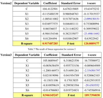
This study utilizes multivariate linear regression to estimate the coefficient of each dependent variable with simulations for the three versions of the system. Simulation results identified three values that explain the significance from the R-square value, F-test statistical value, and t-test score. The R-square value measures how well the linear combination of dependent variable (Xi) predicts independent variable (Y). The F-test confirms the significant correlation between all dependent variables and the independent variable. T-test score verifies the significance of the linear correlation between each dependent variable and the independent variable.
The R-square values for the three versions indicate that the results of linear regression are significant when the values >0.9. The correlation between dependent variables and independent variable is significant when the value is
close to 1 (e.g., version 1, 0.926075805; version 2, 0.917487285; version 3, 0.946145247). That is, the degree of influence for linear combination of dependent variables and the independent variable is strong according when R-square values are high (e.g., in some cases, the relationship is strong when the value is >0.8).
represents two degrees of freedom for SSR and SSE , respectively, as the input for the F-test table). Thus, all
three F-test statistical values exceed the threshold, indicating that the statistical correlations are significant.
Table 5 The result of linear regression for version 1
Version1 Dependent Variable Coefficient Standard Error t-score
C 104.0407841 5.917149646 17.58292257
X1 -1.068432409 0.899405452 -1.18793188
X2 -0.549421368 0.471157987 -1.166108571
X3 -0.027321433 0.043518071 -0.627818108
X4 0.226899222 0.191366761 1.185677286
X5 -7.99108019 0.324059961 -24.65926421
X6 -0.048351515 0.017412681 -2.776799044
R-square 0.926075805 F-test 135.2956055
The t-test score is utilized for verifying the linear correlation between each dependent variable and the independent variable. The threshold for t-test score is 1.6741162 based on a 0.05 (α) value for significance and 53 for the SSE.. Experimental results indicate that X2 and X5 have a significant linear correlation with Y in versions 2 and 3; conversely, X5 and X6 have a linear correlation
with Y for version 1. This correlation is negative, meaning the result is low when the coefficient value is high. The simulation results confirm the assumption that X2 (number of services in the version) and X5 (satisfaction) affect Y (unselected decision score) significantly. Conversely, X6 (profit) affects Y significantly instead of X2 for version 1.
Table 6 The result of linear regression for version 2
Version2 Dependent Variable Coefficient Standard Error t-score
C 104.4122501 6.678215805 15.63475232
X1 -0.115488339 0.986948763 -0.117015537
X2 -1.085411002 0.517071636 -2.099150151
X3 0.034977575 0.046401111 0.753808994
X4 0.06536037 0.211140252 0.309559022
X5 -8.984154346 0.382335077 -23.49811692
X6 0.01204494 0.018842907 0.63922942
R-square 0.917487285 F-test 120.0889177
Table 7 The result of linear regression for version 3
Version3 Dependent Variable Coefficient Standard Error t-score
C 105.8689447 6.318621556 16.75506972
X1 -0.085638459 0.955733156 -0.089604989
X2 -1.200146973 0.514091261 -2.334501797
X3 0.021819096 0.041954789 0.520062103
X4 -0.13831106 0.17013855 -0.812931933
X5 -8.810959619 0.299383394 -29.4303552
X6 -0.014706063 0.019724831 -0.745560916
D. Performance Measurement: Recommendations
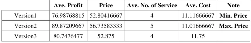
The second performance measurement is the automatic recommendation of the system which is employed to modify the less profitable version in accordance with theorem 3. Based on experimental results, the profits for the three versions are 76.98768815, 89.87209667, and 80.7476477 at prices of 52.80416667, 56.73583333, and 52.875. Version 1, which contains 4 services, has the minimum profit of 52.80416667 for average price, and 11.11666667 for average cost (Table 7-6).
The system is triggered to alter the less profitable version periodically (in 1 or 2 months). Two possible recommendations will be generated based on rules in the knowledge base. The first rule is to recommend a profitable price that is greater than the original price and average price for the three versions (i.e., PV’ > PV* and PV’ > PV, where PV’ is new price, PV is original price, and PV*
is average price). The second rule is to recommend a new price that is between the original price and average price (i.e., PV* > PV’ > PV).
In simulation results, the first recommendation changes the price to 60.03422122 for 6 services in the version; average cost is 10. The new price is higher than the original and average prices (i.e., 60.03422122 > 52.80416667 and 60.03422122 > 54.13833333).
Expected profit for this new price is 87.47910592, which is also greater than original profit of 76.98768815. The new version increases the number of services from 4 to 6 and reduces the cost of the service from 11.11666667 to 10, which is greater than both average and minimum prices, thereby following the rule. This simulation result confirms the theoretical proof of lemma 5, indicating that the profit R is improved when the new price is higher than original and average prices.
Table 8 Detail information for three versions
Ave. Profit Price Ave. No. of Service Ave. Cost Note
Version1 76.98768815 52.80416667 4 11.11666667 Min. Price
Version2 89.87209667 56.73583333 5 11.01666667 Max. Price
Version3 80.7476477 52.875 4 11.75 ġ
An alternative recommendation is provided as another choice. The new price generated is 54.20211534, which is higher than the original price of 52.80416667, but less than the average price of 54.13833333. The new version increases the number of services from 4 to 6, and reduces the cost of the version from 11.11666667 to 9, thereby following the rule stipulating that the price must be greater
than minimum price and less than average price. Expected profit for this new price is 78.73119533, which is also greater than the original profit of 76.98768815. This simulation result verifies the theoretical proof of lemma 6, indicating that profit is improved when the new price is higher than the original average price and less than average price.
Table 9 Automatic recommendations from the system
Recommendation #1
New Price Original Price Ave. Price New No. of
Service
New Ave. Cost
Expected
Profit Note
60.03422122 52.80416667 54.13833333 6 10 87.47910592 >Ave. Price and > Min. Price
Recommendation #2
New Price Original Price Ave. Price New No. of
Service
New Ave. Cost
Expected
Profit Note
54.20211534 52.80416667 54.13833333 6 9 78.73119533 <Ave. Price and > Min. Price
VI DISCUSSION
Simulation results demonstrate that multivariate linear regression confirms the correlation between dependent variables (Xi) and independent variable (Y). The R-square values for the three versions indicate that the degree of influence of the linear combination of dependent variables and the independent variable is strong. All three
F-values are high, revealing that the statistical correlations are significant.
negatively. Profit is also an essential factor (instead of X2) that influences the unselect decision score negatively for version 1.
The system also recommends a new version based on linear regression results. The new price is either higher than the original price of the least profitable version and the average price for the three versions or between these two. Simulation results indicate that the new version is more profitable than the previous one and adjusts the number of services in the version and average cost of services (may increase or decrease the number of services and costs). These simulation results also confirm lemma 5 and lemma 6 of theorem 3 in the economic model, and prove that the proposed approach is feasible.
This study presents a novel automatic rectification approach for less profitable versions periodically. Theorem 3 assumes the new price is has increased profitability, either higher than the original price or average prices of a given version. Simulation results confirm that the new price is most profitable when the system modifies the version with minimum profit routinely.
Multivariate linear regression results indicate that the number of services in a version (in version 2 and version3), satisfaction (in versions 1, 2, and 3), and profits (in version 1) can affect the unselect decision. The system should organize services for each version carefully and follow the rules in the knowledge base. The revised price will be a new version price when the system checks profits during the subsequent time period.
VII CONCLUDING REMARKS
In sum, this work proposes a recommendation-based system to information goods versioning. The recommendation automatically assures the profitable versions that provided from knowledge base. Also, we furnish an economic model and algorithm to prove the feasibility theoretically and practically. The simulation results reveal that the system recommends new version periodically to replace less profitable versions. Finally, this study contributes the impact of three advantages: (1) provides an automatic system to maintain the profits, (2) deliberates the recommendations from knowledge base, and (3) offers an appropriate recommendation to versioning strategy.
REFERENCES
[1]. Banker, R. D., Datar, S. M., Kemerer, C. F., and Zweig, D. (2002) Software Errors and Software Maintenance Management. Information Technology and Management, Vol. 3, pp.25-41.
[2]. Bhargava, H. K. and Choudhary, V., 2001, ‘Information Goods and Vertical Differentiation’, Journal of Management Information Systems, 18, pp. 89-106.
[3]. Hui, K. L. and Chau, Y. K., 2002, ‘Classifying Digital Products’, Communications of the ACM, Vol.45, Iss.6, June, pp. 73 - 79.
[4]. McCain, R. A., 2005, Essential Principles of Economics: A Hypermedia Text. Chapter 16.
[5]. Shapiro, C. and Varian, H. R. (1998) Information Rules; A strategic guide to the network economy, Boston (MA): Harvard Business School Press. [6]. Stigler, G. J., “The Economics of Information,”
Journal of Political Economy, Vol. 69, No. 3, Jun 1961, pp.213-225.
[7]. Sundararajan, A., 2004, ‘Nonlinear Pricing of Information Goods’, 2nd International Industrial Organization Conference, April, pp. 1660-1673. [8]. Sommerville, I. (2000) Software Engineering (6th
edition). Addison Wesley, Chapter 8.
[9]. Ulrich, K. T. and Eppinger, S. D. (1999) Product Design and Development (2nd Edition). McGraw-Hill/Irwin, Chap12.
[10]. Varian, H., “Pricing Information Goods,” Proceedings of the Symposium on Scholarship in the New Information Environment, Harvard Law School, 1995.
[11]. Varian, H., 1997, ‘Versioning Information Goods’, The Economics of Digital Information (tentative), Discussion Paper, Cambridge, MA, MIT Press. [12]. Wang, K. L., “Pricing Strategies for Information