Charge and Current Simulation Method with Boundary Element Method for Grounding System Calculations in Case of Multi- Layer Soil

(1)

e

-ISSN: 2250-3021,

p

-ISSN: 2278-8719

Vol. 3, Issue 6 (June. 2013), ||V4|| PP 14-22

Charge and Current Simulation Method with Boundary Element

Method for Grounding System Calculations in Case of

Multi-Layer Soil

Sherif S. M. Ghoneim

1, 2

_,

IEEE member

1_{Suez University-Egypt,}2_{Taif University, KSA}

Abstract: - Grounding resistance is not only the measurable parameter to give an information about the performance of grounding grids due to discharging current into grounding grids Grounding grids but it is preferable to include the distribution of surface potential and, subsequently, the touch and step voltages over the area above the substation grounding grid and beyond. This paper focuses on the analytical methods to compute not only the Grounding resistance but also the earth surface potential. Three methods are used to compute (Rg)

and (ESP). The first one is the charge simulation method , the second is current simulation method and the last one is the boundary element method (BEM). For BEM, commercial software TOTBEM by university of La Cournia, Spain is used for computing ESP and Rg. The owned Fortran code for the first and second method is

developed to calculate the ESP and Rg. This study is taken into account the type of the soil. In case of grounding

resistance, a comparison between the three methods results and IEEE Standard formula is presented. The results refers that the Fortran code is valid for ESP and Rg calculations.

Index Terms: - Grounding grids, Earth surface potential, Step voltage, Touch voltage, Boundary element method, Charge simulation method, current simulation method.

I. INTRODUCTION

Grounding grids are considered an effective solution for grounding systems for all sites which must be protected from lightning strokes such as, telecommunication towers, petroleum fields, substations and plants. Ground grids are considered complex arrangement and many research efforts have been made to explain the performance of grounding impedance of its under lightning and fault conditions.

The equivalent electrical resistance (Rg) of the system must be low enough to assure that fault currents

dissipate mainly through the grounding grid into the earth, while maximum potential different between close points into the earth’s surface must be kept under certain tolerances (step, touch, and mesh voltages) [1,2]. In a uniform soil, the resistance can be calculated with an acceptable accuracy using several simplifying assumptions [1]. Touch and step voltages are difficult to calculate by simplified method but it determined by analytical expressions [2-5].

Recent papers have proposed new techniques for calculating the earth surface potential and then knowing the step and touch voltages, one of these methods is “A Boundary Element Approach” [6].

Charge and current simulation method help to get good accuracies in field calculation [7-9]. The attractiveness of the charge and current simulation methods, when compared with the other analytical methods such as Finite Element and Finite Difference Methods emanates from its simplicity in representing the equipotential surface of the electrodes, its application to unbounded arrangements whose boundaries extend to infinity and its direct determination to the electric field [10]. The major drawback of the above mentioned methods is that the number, position and the type of replaced simulation charges and current sources and also the position of selected points of writing the equation affect on the accuracy of the method to solve the numerical problems [11]. The other drawback is the difficulty of the application of the method when the number of soil layer increased.

(2)

II. CHARGE SIMULATION METHOD FOR ONE-LAYER SOIL

In the charge simulation method, the actual electric filed is simulated with a field formed by a number of discrete charges which are placed outside the region where the field solution is desired. Values of the discrete charges are determined by satisfying the boundary conditions at a selected number of contour points. Once the values and positions of simulation charges are known, the potential and field distribution anywhere in the region can be computed easily [12].

The basic principle of the charge simulation method is very simple. If several discrete charges of any type (point, line, or ring, for instance) are present in a region, the electrostatic potential at any point C can be found by summation of the potentials resulting from the individual charges as long as the point C does not reside on any one of the charges. Let Qj be a number of n individual charges and Φi be the potential at any point

C within the space. According to superposition principle





n j

j ij i

P

Q

1



(1)

where Pij are the potential coefficients which can be evaluated analytically for many types of charges by solving

Laplace or Poisson’s equations, Φi is the potential at contour (evaluation) points, Qj is the charge at the point

charges.

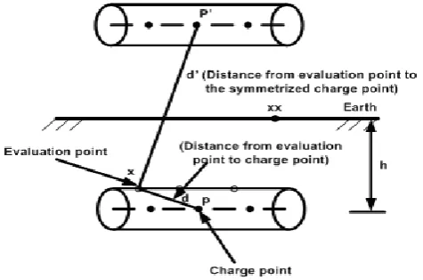
Because of the ground surface is flat, the method of images can be used with the charge simulation method and the potential will be characterized for being constant on the grounding grids and its symmetry [13]. The potential coefficients will be as in the following equation;

















d

P

ij ij ij

'

1

4

1 

(2)

where, dij is the distance between contour point i and charge point j and d’ij is the distance between the contour

point i and image charge point j’ as shown in Figure 1.

As in Figure 1, the fictitious charges are taken into account in the simulation as point charges. The position of each point charges and each contour point are determined in X, Y and Z coordinates where the distance between the contour (evaluation) points are calculated as the following ;



 

2

 

2



2

i j i j i j

ij

X

Y

Z

d













where, Xj, Yj and Zj are the dimensions of the point charge and Xi, Yi and Zi are the dimensions of the contour

point.

After solving equation 1 to determine the magnitude of simulation charges, a number of checked points located on the electrodes where potentials are known, are taken to determine the simulation accuracy. As soon as an adequate charge system has been developed, the potential and field at any points outside the electrodes can be calculated.

The grid is divided into equal segments by the point charges distribution along the axis of grid conductors. Figure 2 shows the distribution of the point charges (dots) for the grounding grid (1 mesh), the number of point charges is distributed on the axis of the grid conductors equally and also the evaluation points distributed on each conductor as shown in Figure 3. The meshes of the grid are always symmetrical.

(3)

Fig. 2:Distribution of point charges on grid

The charge simulation technique is used to get the ground resistance (Rg), ground potential rise (GPR)

and then the surface potential on the earth due discharging impulse current into ground grid is known. The touch and step voltages are calculated from surface potential. The duality expression is used to calculate the ground resistance Rg from the next equation.

1

















C

R

V

Q

C

g n

j j

(3)

where, V is the GPR that is defined 1 V, Qj is the charge of point charge j that used for the calculation, ρ is the

soil resistivity and ε is the soil permittivity.

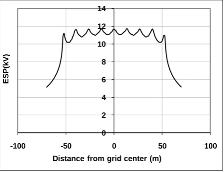
The FORTRAN Code result for the case of study is show in Figure 3. The case study is as follows; Grid area (75m*75m), number of grid meshes 64 meshes, number of point charges 2280, grid depth 0.5m, soil resistivity 2000 ohm.m and the assumed fault current 1000A.

0 2 4 6 8 10 12 14

-100 -50 0 50 100

ESP

(k

V)

Distance from grid center (m)

Fig. 3: ESP for square grid for the case study

(4)

0 2 4 6 8 10 12 14

-100 -50 0 50 100

Dis tance from grid ce nte r (m )

E

S

P

(k

V

)

vertical rod length=0 vertical rod length= 2m

Fig. 4: Effect of vertical rods on ESP

III. CURRENT SIMULATION METHOD IN TWO-LAYER SOIL

The representation of a ground electrode based on equivalent two-layer soil is generally sufficient for designing a safe grounding system. However, a more accurate representation of the actual soil conditions can be obtained by using two-layer soil model [14].

As in the Current Simulation Method, the actual electric filed is simulated with a field formed by a number of discrete current sources which are placed outside the region where the field solution is desired. Values of the discrete current sources are determined by satisfying the boundary conditions at a selected number of contour points. Once the values and positions of simulation current sources are known, the potential and field distribution anywhere in the region can be computed easily [12].

The field computation for the two-layer soil system is somewhat complicated due to the fact that the dipoles are realigned in different soils under the influence of the applied voltage. Such realignment of dipoles produces a net surface current on the dielectric interface. Thus in addition to the electrodes, each dielectric interface needs to be simulated by fictitious current sources. Here, it is important to note that the interface boundary does not correspond to an equipotential surface. Moreover, it must be possible to calculate the electric field on both sides of the interface boundary.

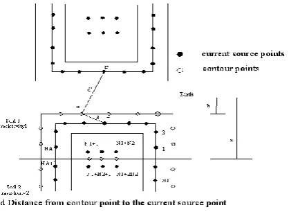
In the simple example shown in Figure 7, there are N1 numbers of current sources and contour points to

simulate the electrode, of which NA are on the side of soil A and (N1- NA) are on the side of soil B. These N1

current sources are valid for field calculation in both soils. At the different soil interface there are N2 contour

points (N1 +1,….., N 1+N2), with N2 current sources (N1+1,…..,N 1+N2) in soil A valid for soil B and N2

current sources (N1+N2 +1,…..,N1 +2N2) in soil B valid for soil A. Altogether there are (N1+N2) number of

contour points and (N1 + 2N2) number of current sources.

As in Figure 5, h is the grid depth and z is the depth of top layer soil. In order to determine the fictitious current sources, a system of equations is formulated by imposing the following boundary conditions.

 At each contour point on the electrode surface the potential must be equal to the known electrode potential. This condition is also known as Dirichlet’s condition on the electrode surface.

 At each contour point on the dielectric interface, the potential and the normal component of flux density must be same when computed from either side of the boundary.

(5)

Thus the application of the first boundary condition to contour points 1 to N1 yields the following equations.

1 1 2,

1 ,

2

1 1, 1 ,

,

1 ...

,

1 ...

2 1 ! 1 2 1 2 ! 1

N

i

V

I

P

I

P

N

i

V

I

P

I

P

A N N N j ij j N

j aij j

A N

N

N N

j ij j N

j aij j



















         (4) where,











 













 













 



' 2 , 2 ' 1 , 1 ' ,

1

4

1

4 ,

1

4 d

d

P

d

P

d

P

j i j i a j i a













Again the application of the second boundary condition for potential and normal current density to contour points = N1+1 to N1+N2 on the dielectric interface results into the following equations. From potential

continuity condition: 2 1 1 2 1 , 1 1 ,

2

0 ....

1 ,

2 1 2 ! 2 1 1

N

i

I

P

I

P

N N N N j j j i N N N j j j

i











       (5)

From continuity condition of normal current density J n:

 

2

 

1 1 2

1

i

J

i

0 for

i

N

1 ,

N

J

_n



_n





(6)

Eqn. (6) can be expanded as follows:

2 1 1 2 1 , 1 1 1 , 2 2 1 , 2 1

,

1 ...

0

1

2 1 2 ! 2 1 ! 1

N

i

I

F

I

F

I

F

N N N N j j j i N N N j j j i N j j j i a

























          



(7) where,







































































































   3 ' ' 3 2 2 , 2 3 ' ' 3 1 1 , 1 3 ' ' 3 ,

4

4 d

zz

d

zz

z

P

F

d

zz

d

zz

z

P

F

d

zz

d

zz

z

P

F

j i j i ij j i j i j i ij j i j i j i a ij a j i a













where, F┴,ij is the field coefficient in the normal direction to the soil boundary at the respective contour point, ρa,

ρ1 & ρ2 are the apparent resistivity and resistivities of soil 1 and 2 respectively and zzi & zzj are the dimension of

the contour point and current source in z direction respectively. Equations 4 to 7 are solved to determine the unknown fictitious current sources.

After solving 4 to 7 to determine the unknown fictitious current source points, the potential on the earth surface can be calculated by using Eq. 4. Also, the ground resistance (Rg) can be calculated using the following

equation:





1 1 N j g

I

V

R

(8)

where, V is the voltage applied on the grid which is assumed 1V.

(6)

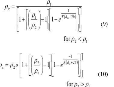
  1 2 2 1 2 1 1

for

1

0





























































 h d K a

e

(9)   1 2 2 1 1 2 2

for

1

0































































  h d K a

e

(10)

where, d0 is the depth to the boundary of the zones, K is the reflection factor (K=( ρ2- ρ1)/ ( ρ1+ ρ2)) and h is the

top layer depth.

Equations 9 and 10 are valid for the boundary depth greater than or equal the grid depth. But in [16], Eq. 10 is modified because at very large depth of upper soil layer, resistivity a given by Eq. 10 tends to 2. This

is physically incorrect if the electrode lies in the upper soil layer, as assumed in [10]. Therefore, Eq. 10 is modified [16] as follows:

  1 2 2 1 1 2 1

for

1

0































































  h d K a

e

(11)

For finite h and very large d0, resistivity a given by Eq. 11 tends to 1, which is in compliance with physical

reasoning.

When the boundary depth is lower than the grid depth, the apparent resistivity tends to 2. Therefore,

by using Eq. 9 and 11 for calculating the grounding resistance by Current Simulation Method, the large different between the proposed method results and the results in [17] is observed for K<-0.5 and this shown in Figure 6. If Eq. 11 is modified as in 12 the results by the proposed method are good agreement with the results in [17].

  1 2 15 1 1 2 1

for

1

0































































  h d K a

e

(12) 0.01 0.1 1 10 100

0.1 1 10 100

T op layer depth (m)

R e si st a n c e ( o h m ) K=0.9 K=0.9-[1] 0.5 K=0.5-[1] 0 K=0-[1] -0.5 K=-0.5-[1] -0.9 K=-0.9-[1]

Fig. 6: Relation between 4 meshes grid resistance and the top layer depth

(7)

0 0.5 1 1.5 2 2.5 3 3.5 4 4.5

-100 -50 0 50 100

E

S

P

(k

V

)

IV. BOUNDARY ELEMENT METHOD

In this section a computer aided design (CAD) system for grounding grids of electrical substations called TOTBEM [6] is presented to get the grounding resistance and earth surface potential. The software code TOTBEM is applied to the case of study as follows;

Grid area (75m*75m), number of grid meshes 64 meshes, grid depth 0.5m, soil resistivity 2000 ohm.m and the assumed fault current 1000A. the result for ESP is shown in Figure 8.

0 2 4 6 8 10 12 14

-150 -100 -50 0 50 100 150

ESP

(k

V)

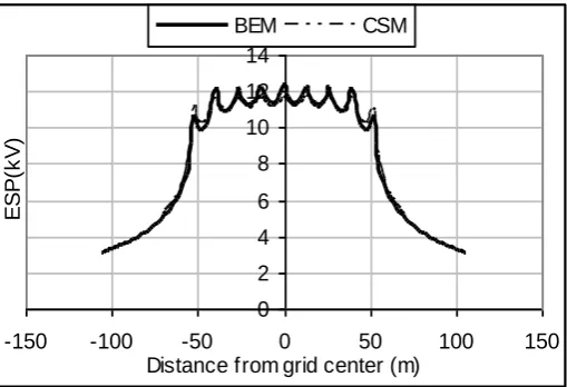
V. COMPARISON BETWEEN THE BEM AND CSM

The following case of study is taken to compare between the results by BEM and CSM, the input data about the grid configuration:

Number of meshes (N) = 64, side length of the grid in X direction (X) = 75m, side length of the grid in Y direction (Y) = 75m, grid conductor radius = 5 mm, vertical rod length (Z) = 0 (no vertical rod), depth of the grid (h) = 0.5 m, resistivity of the soil (ρ) = 2000 Ω.m and the permittivity of the soil is 9.

The following table I explains that the result from the proposed method is close to the other formula in [1] and also the values of resistance that calculated by BEM[6].

TABLE I: Grounding Resistance Between The BEM And CSM And The Other Formulas That Used In IEEE Standards [1]

Rg ohm

Without vertical rods

With vertical rods (2m)

75m*75m 75m*75m

CSM 11.75 11.77

BEM [6] 12.6 12.5

Dwight [1] 11.81 11.8

Laurent [1] 13.29 13.23

Sverak [1] 13.23 13.16

(8)

Figure 9 (a, b) explains that the comparison between CSM and BEM for earth surface potential calculation. The Figure explains that the two methods are close to each other for calculating the ESP although the two methods have different techniques.

0 2 4 6 8 10 12 14

-150 -100 -50 0 50 100 150

Distance from grid center (m)

E

S

P

(k

V

)

BEM CSM

Fig. 9a: Comparison between charge simulation method and Boundary Element Method for 64 meshes (75m*75m) grid without vertical rods (=2000 .m)

0 2 4 6 8 10 12 14

-150 -100 -50 0 50 100 150

Distance from grid center (m )

E

S

P

(k

V

)

BEM CSM

Fig. 9b: Comparison between charge simulation method and Boundary Element Method for 64 meshes (75m*75m) grid with vertical rods 2m and (=2000 .m)

VI. CONCLUSIONS

The three methods charge simulation method, current simulation method and boundary element method that used to calculate the earth surface potential and grounding resistance due to discharging current into grounding grid are efficient. The validation of these methods is satisfying by a comparison between the results from it and the results from the formula in IEEE standard. The charge simulation and current simulation methods give a good agreement with the IEEE standard and with the boundary element method.

REFERENCES

[1] IEEE Guide for safety in AC substation grounding, IEEE Std.80-2000.

[2] J. G. Sverak, “Progress in step and touch voltage equations of ANSI/IEEE Std. 80,” IEEE Trans. Power Delivery, vol. 13, no. 3, Jul. 1999, pp. 762-767.

[3] J. M. Nahman, V. B. Djordjevic, “Nonuniformity correction factors for maximum mesh and step voltages of ground grids and combined ground electrodes,” IEEE Trans. Power Delivery, vol. 10, no. 3, Jul. 1995, pp. 1263-1269.

(9)

[5] S. Serri Dessouki, S. Ghoneim, S. Awad," Ground Resistance, Step and Touch Voltages For A Driven Vertical Rod Into Two Layer Model Soil", International Conference Power System Technology, POWERCON2010, Hangzhou, China, October 2010.

[6] I. Colominas, F. Navarrina, and M. Casteleiro, “Improvement of the computer methods for grounding analysis in layered soils by using high-efficient convergence acceleration techniques” Advances in Engineering Software 44 (2012), pp. 80–91.

[7] E. Bendito, A. Carmona, A. M. Encinas and M. J. Jimenez “The extremal charges method in grounding grid design,” IEEE Transaction on power delivery, Vol. 19, No. 1, January 2004, pp 118-123.

[8] S. Serri Dessouki, S. Ghoneim, S. Awad," Ground Resistance, Step and Touch Voltages For A Driven Vertical Rod Into Two Layer Model Soil", International Conference Power System Technology, POWERCON2010, Hangzhou, China, October 2010.

[9] N. H. Malik, “A review of charge simulation method and its application,” IEEE Transaction on Electrical Insulation, vol. 24, No. 1, February 1989, pp 3-20.

[10] M. Abdelsalam “High voltage Engineering- Theory and Practice”, 2nd edn, 2000.

[11] J. Faiz and M. Ojaghi, "Instructive Review of Computation of Electric Fields using Different Numerical Techniques", Int. J. Engng Ed. Vol. 18, No. 3, 2002, pp. 344±356, printed in Great Britain.

[12] N. H. Malik, “A review of charge simulation method and its application,” IEEE Transaction on Electrical Insulation, vol. 24, No. 1, February 1989, pp 3-20.

[13] E. Bendito, A. Carmona, A. M. Encinas and M. J. Jimenez “The extremal charges method in grounding grid design,” IEEE Transaction on power delivery, vol. 19, No. 1, January 2004, pp 118-123.

[14] Cheng-Nan Chang, Chien-Hsing Lee, “ Compuation of ground resistances and assessment of ground grid safety at 161/23.9 kV indoor/tzpe substation”, IEEE Transactions on Power Delivery, Vol. 21, No. 3, July 2006, pp. 1250-1260.

[15] J. A. Sullivan, “Alternativ earthing calculatons for grids and rods,” IEE Proceedings Transmission and Distributions, Vol. 145, No. 3, May 1998, pp. 271-280.

[16] J. Nahman, I. Paunovic, “Resistance to earth of earthing grids buried in multi-layer soil,” Electrical Engineering (2006), Spring Verlag 2005, January 2005, pp. 281-287.