Comparison of Image Classification Techniques: Binary and
Multiclass using Convolutional Neural Network and Support Vector
Machines
ANUPAMA JAWALE1
GANESH MAGAR2
NARSEE MONJEE COLLEGE OF COMMERCE AND ECONOMICS
PGDEPARTMENT OF COMPUTER SCIENCE,SNDTCOLLEGE [email protected]
Abstract - Classification is the technique applied in data mining to form groups under specified class labels. Classification is supervised type of machine learning. In this paper, two popular classification techniques, Support Vector Machine (SVM) and Convolutional Neural Network (CNN) are compared for accuracy of classification of images. Image classification is done on the basis of feature selection and feature extraction using Tensor flow package. The two classifiers understudy are Linear (SVM) and non-linear techniques (CNN). CNN possesses a powerful feature extraction and SVM is considered as a high-end classifier. Complexity of the feature extraction and selection can be increased in CNN by adding more layers, but in SVM complexity cannot be increased. CNN processes images using matrices of weights and is called as filters or features that detect specific attributes such as vertical edges, horizontal edges, etc. As and when the image progresses through each layer, the filters can recognize more and more complex attributes. In this proposed study, graphs of training phase of CNN also show how the training results are improved image by image due to increasing knowledge of features and thus loss is decreased.
This research study focuses on accuracy measure of the above mentioned methods. For the image classification studied in this paper, it has been observed that SVM gives adequate accuracy for binary classification whereas CNN gives consistent accuracy over binary as well as multi class classification problems. The recognition rate achieved by the CNN algorithm varies between 75% - 75.40 % for binary and multiclass classification. SVM accuracy rate decreases from 80.95 % for binary classification, to 50 % for multiclass classification.
Index Terms- Binary Classification, CNN, Image Dataset, Multi class, SVM, Tensor
(Received November 6st, 2019/ Accepted December 5st, 2019)
I. INTRODUCTION
Image Classification is the crucial issue in machine learning and computer vision. A variety of techniques and methodologies have been proposed for efficient and faster classification [1]. Neural networks have greater potential in the area of image and text processing[2]. For the content based image retrieval, SVM is the proven good performer [3]. However, classification of images and object recognition is a challenging task especially with complex images containing multiple objects. Noise in the image file, availability of various different formats of image file, large size of images make the task more complex.
Color, Texture, Shape etc. are considered as visual descriptors of an image [3]. Color is the most useful information which is in the form of RGB matrix for a raster images. Texture
information is another significant feature , especially for grey scale images [4].
feature extraction typically uses a variety of methods to get a representation of the data and then use the classifier to classify the data.
The two classification techniques presented in this paper can be illustrated as given below
A. Support Vector Machine
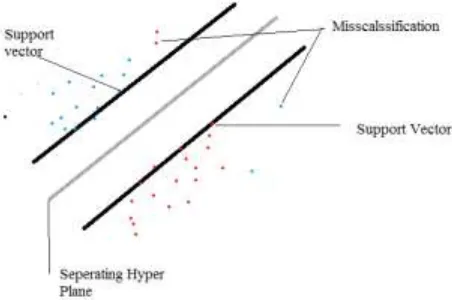
A Support Vector Machine (SVM) is a discriminative classifier formally defined by a separating hyperplane. For the SVM classifier, if a labeled training data is given (supervised learning), the algorithm outputs an optimal hyperplane which categorizes new data items. In two dimensional space this hyperplane is a line dividing a plane in two parts where each class placed in either side. It is a supervised learning method. It is a linear model of classification and regression. According to the SVM algorithm points closest to the line from both the classes are located. These points are called support vectors. Then the distance between the line and the support vectors is computed. This distance is called the margin. SVM aims towards maximization of the margin. The hyperplane for which the margin is maximum is the optimal hyperplane.
Figure 1 : Support Vector Machine Classification
SVM model requires labeled data and accuracy of the model is highly dependent upon the dataset features. In the training process, the algorithm analyzes input data and recognizes patterns and features in a multi-dimensional feature space (hyperplane). All input data items are represented as points in this space, and are mapped to output classes in such a way that classes are divided by as wide and clear gap as possible. For prediction, the SVM algorithm assigns new data item into one category or the other, mapping them into that same space. In the randomly distributed data, where clear definition of hyperplane is not possible, kernel concept can be used to locate a clear class or hyperplane.
For randomly distributed data points, SVM uses ‘kernel’, to specify a method of using linear classifier for solving nonlinear classification problems.
Mathematically, kernel can be defined as
𝑘(𝑥, 𝑦) = 𝑓(𝑥). 𝑓(𝑦) (1)
where, k is the kernel function, x, y are n dimensional inputs. f is a map from n-dimension to m-dimension space such that m>>n.
There are four types of kernels’ functions available with SVM function as given below.
Table 1: Kernels and their representative formula
Kernel Function Formula
Linear u'v
Polynomial (γμ'ϑ+coef0)degree
Radial e(-γ|μ-ϑ|2
Sigmoid tanh (γμ'ϑ +coef0) [7]
In this experiment, we have used ‘radial’ method for kernel definition. A Radial Basis Function defined above is the real valued function whose value depends only upon the distance from the origin. The distance is usually the ‘Euclidian distance’. The basic principle of SVM is to maximize the distances of samples to a boundary that separates the classes. This principle makes SVM suitable for a 2-class problem. But SVM’s can also be used for multi-classification, by combining multiple 2-class SVM’s, as described in the later section. SVM employs kernel tricks and maximal margin concepts to perform better for non-linear and high-dimensional tasks like image dataset. For images, Multilevel wavelet decomposition can also be applied for larger datasets to increase classification accuracy and computation time performance improvement [1].
To evaluate performance of SVM algorithm on given dataset, two metrics can be used, viz, Accuracy Metric and Kappa Value Metric.
i. Accuracy is the percentage of correctly classifies instances out of all instances. It is more useful on a binary classification than multi-class classification problems.
ii.
Kappa or Cohen’s Kappa is like classification accuracy, except that it is normalized at the baseline of random chance on the dataset. It is a more useful measure to use on problems that have an imbalance in the classes.B. Convolution Neural Network (CNN)
Convolutional neural networks consider and process images as tensors [9]. Tensors are matrices of numbers with additional dimensions. A tensor’s dimensionality (1, 2, 3…n) is known as order of the tensor.
Height and width of a single image, determines 2 row-col dimensions whereas its R-G-B- values define additional 3 layers of the image. Each layer is called as a channel.
In image analysis performed by CNN model, first the input image is being analyzed, and then filtered. Filtration include feature extraction of the image. The two functions relate to each other by multiplication. A convolution is the integral measuring how much two functions overlap as one passes over the other. The purpose of convolution layer is to receive a feature map. It starts with low number of filters for low-level feature detection. The deeper it goes into the CNN, the more filters are used to detect high-level features. In the process of feature extraction, convolutional nets pass many filters over a single image, each one picking up a different signal. Convolutional networks take those filters, slices of the image’s feature space, and map them one by one; that is, they create a map of each place that feature occurs. By learning different portions of a feature space, convolutional nets allow for easily scalable and robust feature engineering.
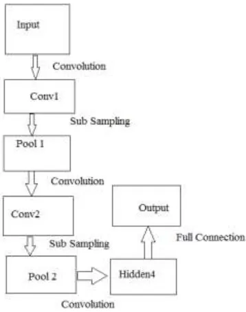
For image analysis and feature extraction, Convolutional Neural Networks made up of neurons that have learnable weights and biases receives some inputs, performs a dot product and optionally follows it with a non-linearity. The whole network still expresses a single differentiable score function from the raw image pixels on one end to class scores at the other. This process can be shown as per below flow diagram
Figure 2 : Flow of Convolution Neural Network
Convolutional networks are designed to reduce the dimensionality of images in a variety of ways [10], [11]. One way is Filter Stride while other way is down sampling. Next to convolution, max pooling, down sampling and subsampling occur. The activation maps are fed into a down sampling layer, and like convolutions, this method is applied one patch at a time. For example, max pooling simply takes the largest value from one patch of an image, places it in a new matrix next to the max values from other patches, and discards the rest of the information contained in the activation maps. Overall the CNN based methods have better performance than hand-crafted features based methods[12].
In this study, CNN classification are implemented using the Tensorflow library. Tensorflow is an open-source software library developed by the Google for numerical computation [13].
II.EXPERIMENTAL WORK
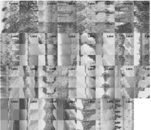
For the experiments discussed in this paper, the image data set
is downloaded from Sun Database
(https://groups.csail.mit.edu/vision/SUN/) that contains 4970 images of Forest, Lake and Buildings. Images are in jpg format. All images are label uniquely to describe their contents.
Using R Studio release 3.5.3 SVM and CNN algorithms are implemented and tested for the accuracy of classification. SVM is first used for Binary Classification and later used for multi class (3 classes) classification. It can be used to carry out general regression and classification, as well as density-estimation. List of different parameters used for SVM implementation is given below.
i. Parameters: SVM-Type, Value : C-classification For this type of SVM, training involves the minimization of the error function:
1
2w
T+C∑N ℵ
i=1 (2)
Where C is the capacity constant, w is the vector of coefficients, and ℵ represents parameters for handling non separable data (inputs). The index i labels the N training cases
ii. Parameter SVM-Kernel, Value : Radial As mentioned in Table 1 above
This parameter is needed for all kernels except linear kernel. Its default value is 1/(data dimension) Gamma is the free parameter of the Gaussian radial basis function (Refer to Table 1)
Smaller value of Gamma indicates the class of x support vector will have influence on deciding the class of the vector y even if the distance between them is large. Large gamma value indicates high bias and low variance models.
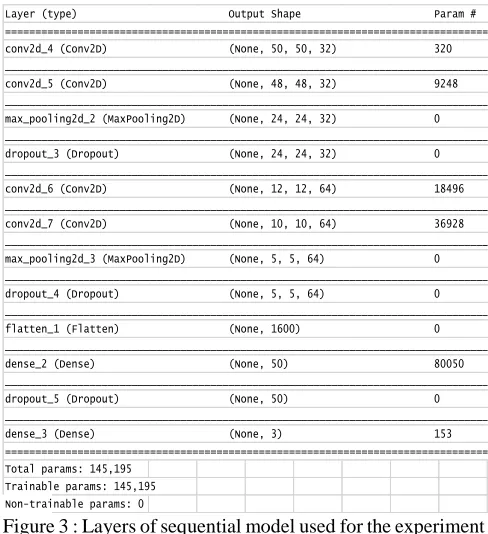
For implementation of CNN, library ‘Keras’ is used. It is user friendly neural network library written in Python [14]. Tensorflow is one of the packages in library keras, which has the best performance for image classification in python [15]. We can import this library to R to use classification model defined in it. The model we define with ‘keras’ is a sequential model. Sequential model is built layer by layer [16]. Each layer has a weight that correspond to next layer.
Below figure shows different layers of Sequential Model
Figure 3 : Layers of sequential model used for the experiment i. Dense is a standard layer [17] type that works for most
cases. In a dense layer, all nodes in the previous layer connect to the nodes in the current layer. Dense layer implements ‘output = activation(dot(input, kernel) + bias)’ where activation is the element-wise activation function passed as the activation argument, kernel is a weights matrix created by the layer, and bias is a bias vector created by the layer. The first layer in a model must have ‘input_shape’ defined.
ii. Dropout consists in randomly setting a fraction rate of input units to 0 at each update during training time, which helps prevent over fitting.
iii. Flatten layer flattens the input.
iv. Max pooling operation defines pooling process for spatial data [18].
v. Conv2D layer creates a convolution kernel that is convolved with the layer input to produce a tensor of outputs. If ‘use_bias’ is true, a bias vector is created and added to the outputs.
vi. ‘ReLU’ activation function returns 0 for every negative value in the input image while it returns the same value for every positive value.
III.RESULTS DISCUSSION AND INTERPRETATION
The outcome of the research work on the basis of experiments can be presented as below.
Table 2 : Support Vector Machine for Binary Classification
Accuracy : 0.8095 95% CI : (0.6909, 0.8975) No Information Rate : 0.5079
P-Value [Acc > NIR] : 6.935e-07
Kappa : 0.6209
Mcnemar's Test P-Value : 0.009375
Sensitivity : 0.6562 Specificity : 0.9677 Pos Pred Value : 0.9545 Neg Pred Value : 0.7317 Prevalence : 0.5079 Detection Rate : 0.3333 Detection Prevalence : 0.3492 Balanced Accuracy : 0.8120
'Positive' Class : 0
Layer (type) Output Shape Param # ==================================================================================== conv2d_4 (Conv2D) (None, 50, 50, 32) 320 ____________________________________________________________________________________ conv2d_5 (Conv2D) (None, 48, 48, 32) 9248 ____________________________________________________________________________________ max_pooling2d_2 (MaxPooling2D) (None, 24, 24, 32) 0 ____________________________________________________________________________________ dropout_3 (Dropout) (None, 24, 24, 32) 0 ____________________________________________________________________________________ conv2d_6 (Conv2D) (None, 12, 12, 64) 18496 ____________________________________________________________________________________ conv2d_7 (Conv2D) (None, 10, 10, 64) 36928 ____________________________________________________________________________________ max_pooling2d_3 (MaxPooling2D) (None, 5, 5, 64) 0 ____________________________________________________________________________________ dropout_4 (Dropout) (None, 5, 5, 64) 0 ____________________________________________________________________________________ flatten_1 (Flatten) (None, 1600) 0 ____________________________________________________________________________________ dense_2 (Dense) (None, 50) 80050 ____________________________________________________________________________________ dropout_5 (Dropout) (None, 50) 0 ____________________________________________________________________________________ dense_3 (Dense) (None, 3) 153 ==================================================================================== Total params: 145,195
Figure 4 : Screenshot of actual output of Binary Classification by SVM (Lake , Forest)
Accuracy : 0.8095
95% CI : (0.6909, 0.8975) No Information Rate : 0.5079 P-Value [Acc > NIR] : 6.935e-07 Kappa : 0.6209 Mcnemar's Test P-Value : 0.009375 Sensitivity : 0.6562 Specificity : 0.9677 Pos Pred Value : 0.9545 Neg Pred Value : 0.7317 Prevalence : 0.5079 Detection Rate : 0.3333 Detection Prevalence : 0.3492 Balanced Accuracy : 0.8120 'Positive' Class : 0
Table 3: Support Vector Machine Multiclass (3 Classes) Classification
Accuracy : 0.5
95% CI : (0.2822, 0.7178) No Information Rate : 0.3636 P-Value [Acc > NIR]: 0.1346
Kappa : 0.2644
Mcnemar's Test P-Value : 0.0719 Statistics by Class:
Class: 0
Class: 1
Class: 2
Sensitivity 0.7143 0.7143 0.12500 Specificity 0.5333 0.7333 1.00000 Pos Pred Value 0.4167 0.5556 1.00000 Neg Pred Value 0.8000 0.8462 0.66667 Prevalence 0.3182 0.3182 0.36364 Detection Rate 0.2273 0.2273 0.04545 Detection Prevalence 0.5455 0.4091 0.04545 Balanced Accuracy 0.6238 0.7238 0.56250
Figure 5 : Screenshot of actual output of Multiclass Classification by SVM (Lake, Forest, Building)
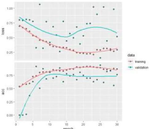
Figure 6 : Graph for comparison for first 30 iterations : Training Accuracy & Loss , Validation Accuracy and Loss – Binary Classification
Figure 7 : Graph for comparison for first 30 iterations : Training & Validation Accuracy & Loss Line graph – Binary Classification
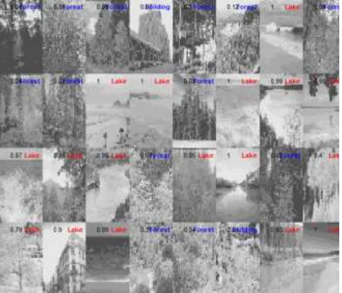
Figure 8 : Screenshot of actual output of Binary Classification by CNN (Lake, Forest)
Convolution Neural Network Model for Multiclass (3 Classes) Classification
Figure 10 : Graph for comparison for first 30 iterations : Training & Validation Accuracy & Loss Line graph – Multiclass Classification
Figure 8 : Screenshot of actual output of Multi value Classification by CNN (Lake, Forest)
Table 4 : Comparison of SVM and CNN for accuracy of classification
Classification Method Accuracy %
Support Vector Machine Binary
Classification 80.95%
Support Vector Machine Multiple Class
Classification 50%
Convolution Neural Network Binary
Classification 75%
Convolution Neural Network Multiple Class
Classification 78.4%
IV. CONCLUSION
This study shows that Support Vector Machine is the better choice of algorithm to achieve accuracy in binary image classification (80.95%). Convolution Neural Network shows consistency in accuracy for binary as well as multiple class classification. In both the cases, CNN shows 75 and 78.4 % accuracy. Accuracy of SVM for multiclass classification is less (50%) which can be improved by adding feature selection steps to the original algorithm. This may be viewed as future scope of the study.
Also, computation speed for both the algorithms can be improved on multi core parallel environment. Same study can be performed for varied number of layers in CNN model.
V. REFERENCES
[1] B. Demir and S. Ertrk, “Improving SVM classification accuracy using a hierarchical approach for hyperspectral images,” in 2009 16th IEEE International Conference on Image Processing (ICIP), Cairo, 2009, pp. 2849–2852. [2] R. Lippmann, “An introduction to computing with neural
nets,” IEEE ASSP Mag., vol. 4, no. 2, pp. 4–22, 1987. [3] N. Boujemaa and K. Khaldi, “Images research by
content,” in 2019 International Conference on Computer and Information Sciences (ICCIS), Sakaka, Saudi Arabia, 2019, pp. 1–5.
[4] T. Ojala, M. Pietikainen, and T. Maenpaa,
“Multiresolution gray-scale and rotation invariant texture classification with local binary patterns,” IEEE Trans. Pattern Anal. Machine Intell., vol. 24, no. 7, pp. 971–987, Jul. 2002.
[5] P. Viola and M. Jones, “Rapid object detection using a boosted cascade of simple features,” in Proceedings of the 2001 IEEE Computer Society Conference on Computer Vision and Pattern Recognition. CVPR 2001, Kauai, HI, USA, 2001, vol. 1, pp. I-511-I–518.
[6] A. Vailaya, A. Jain, and Hong Jiang Zhang, “On image classification: city vs. landscape,” in Proceedings. IEEE Workshop on Content-Based Access of Image and Video Libraries (Cat. No.98EX173), Santa Barbara, CA, USA, 1998, pp. 3–8.
[7] H.-T. Lin and C.-J. Lin, “A Study on Sigmoid Kernels for SVM and the Training of non-PSD Kernels by SMO-type Methods,” p. 32.
Advanced Image Technology (IWAIT), Chiang Mai, 2018, pp. 1–4.
[9] D. Demirovic, E. Skejic, and A. Serifovic-Trbalic, “Performance of Some Image Processing Algorithms in Tensorflow,” in 2018 25th International Conference on Systems, Signals and Image Processing (IWSSIP), Maribor, Slovenia, 2018, pp. 1–4.
[10] N. Yi, C. Li, X. Feng, and M. Shi, “Research and
Improvement of Convolutional Neural Network,” in 2018 IEEE/ACIS 17th International Conference on Computer and Information Science (ICIS), Singapore, 2018, pp. 637–640.
[11] P. M. Krishnammal and S. S. Raja, “Convolutional Neural Network based Image Classification and Detection of Abnormalities in MRI Brain Images,” in 2019 International Conference on Communication and Signal Processing (ICCSP), Chennai, India, 2019, pp. 0548–0553.
[12] L. Lu, Y. Yi, F. Huang, K. Wang, and Q. Wang, “Integrating Local CNN and Global CNN for Script Identification in Natural Scene Images,” IEEE Access, vol. 7, pp. 52669–52679, 2019.
[13] F. Ertam and G. Aydin, “Data classification with deep learning using Tensorflow,” in 2017 International Conference on Computer Science and Engineering (UBMK), Antalya, 2017, pp. 755–758.
[14] P. Vidnerová and R. Neruda, “Evolving KERAS
Architectures for Sensor Data Analysis,” presented at the 2017 Federated Conference on Computer Science and Information Systems, 2017, pp. 109–112.
[15] R. Phadnis, J. Mishra, and S. Bendale, “Objects Talk - Object Detection and Pattern Tracking Using
TensorFlow,” in 2018 Second International Conference on Inventive Communication and Computational Technologies (ICICCT), Coimbatore, 2018, pp. 1216– 1219.
[16] J. L. Ziegler, R. T. Arn, and W. Chambers, “Modulation recognition with GNU radio, keras, and HackRF,” in 2017 IEEE International Symposium on Dynamic Spectrum Access Networks (DySPAN), Piscataway, NJ, 2017, pp. 1–3.
[17] K. He, X. Zhang, S. Ren, and J. Sun, “Deep Residual Learning for Image Recognition,” in 2016 IEEE
Conference on Computer Vision and Pattern Recognition (CVPR), Las Vegas, NV, USA, 2016, pp. 770–778. [18] J. B. L. Iv, Z. Zhou, C. Zhang, P. Gong, and Y. Zhang,