Journal of Nature and Science, Vol.1, No.7, e130, 2015 Physical Sciences
Using the Tractometer to assess performance of a new statistical
tractography techniqu
e
Lyudmila Sakhanenko*
Department of Statistics and Probability, Michigan State University, East Lansing, MI 48824, USA
We evaluate a recent statistical tractography technique for analyzing the diffusion tensor imaging data using new criteria and the template from the Tractometer. This novel method simultaneously achieves excellent percentages on 3 out of 7 criteria. Compared to deterministic tractography methods, it is superior to all of them. Compared to probabilistic tractography methods, it has similar results for so-called ABC metric and better performance for all the other metrics. On top of this, it is faster and it additionally provides more geometrical information through confidence ellipsoids rather than through a bundle of repeated tracts. Journal of Nature and Science, 1(7):e130, 2015
integral curve | tractography | diffusion tensor imaging
How to cite this article? Here is an example:
Sakhanenko L (2015) Using the Tractometer to assess performance of a new statistical tractography technique. Journal of Nature and Science, 1(7):e130.
This is title page, followed by full text + 4 figures (12 pages)
Conflict of interest: No conflicts declared.
*
Corresponding Author. Department of Statistics and Probability, Michigan State University, East Lansing, MI 48824-1027, USA. Email: [email protected]
Using the Tractometer to assess performance of a new
statistical tractography technique
Lyudmila Sakhanenko
∗Michigan State University
June 10, 2015
Journal of Nature and Science, Vol.1, No.7, e130, 2015
Abstract
We evaluate a recent statistical tractography technique for analyzing the diffu-sion tensor imaging data using new criteria and the template from the Tractometer.
This novel method simultaneously achieves excellent percentages on 3 out of 7 crite-ria. Compared to deterministic tractography methods, it is superior to all of them. Compared to probabilistic tractography methods, it has similar results for so-called
ABC metric and better performance for all the other metrics. On top of this, it is faster and it additionally provides more geometrical information through confidence ellipsoids rather than through a bundle of repeated tracts.
Key words: integral curve, tractography, diffusion tensor imaging
1
Introduction
Recently Carmichael and Sakhanenko (2014) proposed a new statistical technique (which we will call CS method below for brevity) for estimating integral curves driven by the dominant eigenvector field of a tensor field, whose components are slopes in a system of regression equations. They use kernel smoothing to estimate tensor components, then take the field of the main eigenvectors of the estimated tensor field, and trace the integral curves along this vector field in small steps. In essence, the integral curve estimator is a plug-in estimator based on kernel smoothing of the tensor field. They showed theoretically
∗Department of Statistics and Probability, East Lansing, MI 48824-1027, [email protected]. Research
that these estimators are asymptotically normal under certain regularity conditions on the underlying tensor field. The asymptotical variance of the estimator and its bias can be estimated together with the estimator in small steps sequentially. Geometrically the results are presented by an estimated curve together with confidence ellipsoids along it, see an example in Figure 1 (a). One can easily assess how the uncertainty in image components has propagated to the trajectory, and how it changes as the curve goes through regions of higher uncertainty levels such as near branching points. This tractography method is motivated by and used for estimation of neural fibers in a brain from a dataset of observed noisy diffusion tensor imaging (DTI) components; see the model in the next section.
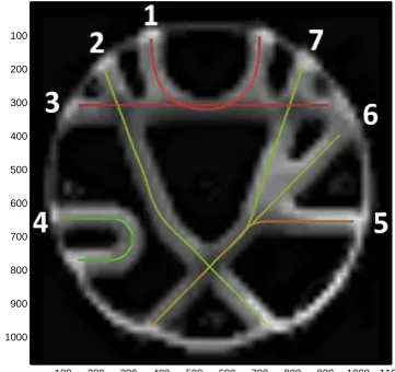
There are many different tractography methods for DTI, a popular en vivo brain imaging technique; see Assemlal et.al. (2011) for a complete review. However, the comparison of them is tricky. First, there is no agreement on a golden standard in simulated studies or in real scans. Secondly, the methods are designed to achieve different goals. For example, some model the tensor field or the vector field while tracing of the fibers is secondary. Recently Cˆot´e et.al. (2013) attempted to alleviate this problem and proposed a novel evaluation system for tractography methods. It is based on an artificial template which we reproduce from their website in Figure 1 (b). It mimics the typical behavior of neural fibers. Then they select a set of metrics used for quantitative assessment of the methods. These metrics are average bundle coverage (ABC), valid connections (VC), invalid connections (IC), no connections (NC), valid bundles (VB), and invalid bundles (IB). They are motivated by needs of human brain imaging practitioners. The metrics target the global connectivity. It is the first systematic attempt to go from a qualitative comparison to a quantitative one.
They also collect various approaches into a database, which are then rated based on the metrics. A recent summarized report can be found in Daducci et.al. (2013). The goal of this paper is to compare the method of CS against others using Tractometer and also to show how the selected metrics might not do justice to statistical tractography methods.
2
Model and algorithm
At a fixed location xin a 3D regionGwe assume that the observationsY(x)∈RN, N ≥6,
arise from a mixture of two underlying tensors M(1)(x) and M(2)(x),which have the same
simple maximal eigenvalue but different leading eigenvectors v(M(1)(x)) and v(M(2)(x)) : Y(x) =B(πM(1)(x) + (1−π)M(2)(x)) + Σ1/2(x)Ξx. (1)
Here the symmetric tensors M(i)(x), i = 1,2, are represented by 6D vectors, B is a fixed
co-variance matrix. Σ(x) is a positive definite 6×6 unknown matrix. The mixing coefficientπ
determines the relative contributions ofM(1)(x) andM(2)(x) toY(x).A variety of standard
clustering techniques can be applied to estimate M(1)(x) and M(2)(x) as well as π. In our
simulation study we use the standard clustering procedures based on the mixture of two Gaussian distributions.
The model (1) is motivated by low angular resolution DTI. It is based on measurements of water diffusion on a grid of points. Locally the relative amount of water diffusion along a spatial direction b∈R3, ∥b∥= 1,at a voxel x, S(x, b), is estimated as follows:
log
(
S(x, b)
S0(x)
)
=−cb∗D(x)b+σ(x, b)ξb,
where S0(x) is the amount of water diffusion without gradient application; σ(x, b)>0; ξb
describes noise; the constantcdepends only on the proton gyromagnetic ratio, the gradient pulse sequence shape, duration and other timing parameters of the imaging procedure; D
is a 3×3 symmetric positive definite matrix. On practice a set of N directions b is chosen and the corresponding log-losses are measured. They are stacked into a vector-column
Y in the model (1). Meanwhile the upper triangular part of matrix D is stacked into a 6D vector-column M. We remark that the mixture of tensors is used to model branching phenomenon.
Now we observe a set of Y(xj), j = 1, ..., n, for a collection of sites xj, j = 1, ..., n,
in G, which usually forms a 3D grid. CS method first takes the least squares estimators ˜
Mn(xj) for πM(1)(xj) + (1−π)M(2)(xj) at each grid pointxj, j = 1, ..., n,and smooths the
tensor field using kernel regression estimation to obtain the estimated tensor field ˆMn(·)
everywhere in the region G. Also at each xj the clustering is done if the Gaussian mixture
test finds more than 1 cluster. Secondly, taking into account the clusters, the tracing of the estimated integral curve ˆXn(·) is done in small stepsδ >0 in the direction of the dominant
eigenvector field v(M(i)(x)), x∈G, i= 1,2.Approximation to the asymptotical covariance
matrix C(·) and the bias µ(·) of the estimated curve are also calculated on each step from the previous step values because they do not require the knowledge of the whole trajectory
x(t), t∈[0, T].
For completeness we list the steps of the algorithm for one cluster. 1. Initialize q= 0, tq = 0,Xˆn(t0) = x0, µ(t0) = 0, C(t0) = 0.
small steps tq=qδ, q= 0,1,2, ...
˜
Mn(xj) = (B∗B)−1B∗Y(xj), j = 1, ..., n, Mˆn(x) =
1 nh3 n n ∑ j=1 K (
x−xj hn
)
˜
M(xj),
ˆ
Xn(tq) = ˆXn(tq−1) +δv( ˆMn( ˆXn(tq−1))).
Here B∗ stands for the transpose of B; v(A) denotes the main eigenvector of matrix
A; K is a symmetric about 0, probability density with a finite second moment, for example the standard Gaussian density in 3D; the averaging window (bandwidth) size ishn = (β/n)1/6 with some finite pre-selected constant β >0.This tuning parameter
can be chosen as the minimizer of the mean integrated squared error (MISE) between the estimated and the true integral curves as proposed in Carmichael and Sakhanenko (2014). Then β = 0.25(d −1)∫0T trC(t, t)dt[ ∫0Tµ1(t)∗µ1(t)dt
]−1
, where one uses
β = 1 in µ1. One would start with an initial β, estimate µ1 and C accordingly,
re-evaluate β based on these µ1 and C, and repeat.
3. Approximate the gradient of the tensor field by ∇Mˆn(x), the tensor of second order
derivatives of the tensor field by∇2Mˆ
n(x) and covariance matrix of the noise by ˆΣn(x)
using the following formulas: for j = 1, ..., n
˜
Σn(xj) =
1
m−1
m ∑
i=1
(Y(Li)−BM˜(Li)−Y¯ +BM¯˜)(Y(Li)−BM˜(Li)−Y¯ +BM¯˜)∗,
where Li, i = 1, ..., m, are the measurement locations in a local neighborhood of xj
and the averages ¯Y andM¯˜ are taken over themvaluesY(Li) and ˜M(Li),i= 1, ..., m,
respectively. For instance, for a regular 3D gridxj, j = 1, ..., n,we could set theLi to
be the points in the cube of 26 immediate neighbors surrounding xj in all 3 spatial
directions. Then for x∈G
ˆ
Σn(x) =
1 nh3 n n ∑ j=1 K (
x−xj hn
)
˜ Σn(xj),
∇Mˆn(x) = 1
n˜h4 n n ∑ j=1 ∇K (
x−xj
˜
hn )
˜
M(xj), ˜hn = (
logn n
)1/4 ,
∇2Mˆ n(x) =
1
n˜˜h5 n
n ∑
j=1
∇2K
(
x−xj
˜ ˜
hn )
˜
M(xj), ˜˜hn = (
logn n
)1/5 .
components: for 1≤p, k, l ≤3
∂vp( ˆMn(x)) ∂Mkl
= (1−0.5δkl) [
(λ( ˆMn(x))Id−Mˆn(x))+pkvl( ˆMn(x))
+(λ( ˆMn(x))I−Mˆn(x))+plvk( ˆMn(x)) ]
,
where A+ stands for the Moore-Penrose inverse of a matrix A and λ(A) denotes the
eigenvalue of A. Here I is the 3×3 identity matrix and δkl = 0 for k ̸= l and 1 for k =l.
5. Approximate the asymptotical biasµ(tq), q≥1, as
ˆ
µ(tq) = ˆµ(tq−1) +δ∇v( ˆMn( ˆXn(tq−1)))∇Mˆn( ˆXn(tq−1))ˆµ(tq−1)
+0.5δ√β∇v( ˆMn( ˆXn(tq−1)))
∫
R3
K(z)⟨∇2Mˆn( ˆXn(tq−1))z, z⟩dz.
6. Approximate the asymptotical covarianceC(tq), q≥1, as
ˆ
C(tq) = ˆC(tq−1)
+δ∇v( ˆMn( ˆXn(tq−1)))∇Mˆn( ˆXn(tq−1)) ˆC(tq−1)
+δCˆ(tq−1)∇Mˆn( ˆXn(tq−1))∗∇v( ˆMn( ˆXn(tq−1)))∗
+δψ(v( ˆMn( ˆXn(tq−1)))) ˜∇v( ˆMn( ˆXn(tq−1)))
×[ ˆMn( ˆXn(tq−1)) ˆMn∗( ˆXn(tq−1)) + ˆΣn( ˆXn(tq−1))]
×∇v( ˆMn( ˆXn(tq−1)))∗,
where ψ(v) =∫R∫R3K(z)K(z+τ v)dzdτ.
7. Approximate the 100(1−α)% confidence ellipsoid for x(tq), q≥1,as
P{Cˆ(tq)−1/2 (√
nh2
n( ˆXn(tq)−x(tq))−µˆ(tq) )
≤Rα }
≈1−α,
where P(|Z| ≤Rα) = 1−α for a standard normal 3D vector Z.
8. Repeat steps 2–6 untiltq reaches T.
3
Simulation results
use this approach since in DTI model Rician noise at typical noise-to-signal ratios is well approximated by Gaussian noise; see for example discussion in Zhu et.al. (2007). Before estimation we performed the standard clustering test at each voxel xj and identified
loca-tions where the test found 2 significant clusters of tensors M(1) andM(2). Then near these
locations we clustered the tensor field and performed the whole technique separately in each cluster, that is the kernel smoothing was applied to estimated ˆMn(i), i= 1,2,separately,
fol-lowed by finding the fields of main eigenvectors and tracing 2 fibers. To our dismay adding clustering did not dramatically change the performance of CS method. We even tried to go to an extreme and forced clustering at each voxel. In this case the global connectivity metrics got worse, the frequency of fibers going off the template and just stopping increased significantly.
For each curve on the template we started its tracing at a point in the regions of interest at both ends. The tracing of curve 1 is good. One direction gives better results than when we start from the other end region. The method fails to trace the complete curve 2. We varied the initial point inside both end regions and the tracing was unstable. When starting from one end it tends to go into curve 3, from the opposite end it goes into curve 5. The tracing of curve 3 is also unstable. When we varied the initial point from one end curve 3 tends to go into curve 2 and then into curves 5-6-7. Starting from the opposite end it goes into curve 7. The tracing of curve 4 is good. One direction gives better results for the confidence ellipsoids than when we start from the other end region. Curves 5-6-7 go together when started from left end region. Curve 5 starts ok but at the end it turns into curve 2. The tracing of curve 6 is good. Starting at any endpoint yields equally good results with tight confidence ellipsoids. Curve 7 either immediately turns into curve 3 or goes ok till it meets with curve 2 where it turns into it. To summarize curves 2, 3, 5, and 7 present the most challenge for CS method. Figure 4 illustrates what happens when the initial point varied in the end regions of these curves. Let us stress that unlike probabilistic tractography methods outputs, these tracks are not realizations of a random procedure. They are different because the initial point is different, leading to different averaging windows moving along the estimated curve. Again we stress that if the method is repeated for the same dataset with the same initial location and the same parameters (K, hn, β) it results in the same estimated curve with the same confidence ellipsoids. Thus,
ABC and PC for curves 1, 4, and 6 are 100% and they are 0% for curves 2, 3, and 5. Since curve 7 is recovered ok if the tracing starts from one endpoint but not from the other, ABC and PC are 50%.
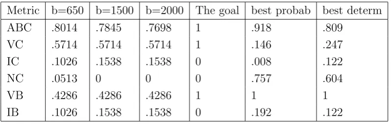
Metric b=650 b=1500 b=2000 The goal best probab best determ ABC .8014 .7845 .7698 1 .918 .809
VC .5714 .5714 .5714 1 .146 .247 IC .1026 .1538 .1538 0 .008 .122
NC .0513 0 0 0 .757 .604
VB .4286 .4286 .4286 1 1 1 IB .1026 .1538 .1538 0 .192 .122
Table 1: Metrics from the Tractometer evaluated for CS method. Columns ”the best probab” and ”best determ” contain the best values for each metric by different methods from Cˆot´e et.al. (2013). The column ”the goal” gives the best desired levels of each metric.
data with 3 different levels of noise b = 650,1500,2000 s/mm2 given on the Tractometer
website. As expected, the confidence ellipsoids became wider and covered more volume. For example, along curve 4 the norms of the ellipsoids increase by an approximate factor 2 when we switch from b = 650 to b = 1500, and by approximately 1.5 when we go from
b = 1500 to b= 2000.
Finally, we consider the metrics proposed in the Tractometer. The overall results are summarized in Table 1. For average bundle coverage (ABC) we consider one estimated trajectory together with the 95% confidence ellipsoids along it in place of the bundle of trajectories usually produced by a probabilistic tractography method. Valid connections (VC), valid bundles (VB) and invalid bundles (IB) are calculated as ratios out of 7. Invalid connections (IC) and no connections (NC) are calculated as ratios out of 39. The numbers for the best probabilistic and best deterministic methods are taken from the paper of Daducci et.al. (2013).
4
Discussion and conclusion
CS method does not recover 7/7 VB but it simultaneously achieves high ABC of 80.14%, high VC of 57.14% and low IB 6/39. If one compares it against deterministic tractography methods, it is superior to all of them. If one compares it against probabilistic tractography methods, it has comparable results for ABC metric and better for all the other metrics. But it is faster and additionally provides more geometrical information through confidence ellipsoids rather than through a bundle of repeated tracts.
Note that the comparison metrics in Tractometer are mainly image-based rather than geometry-based. Meaning that for example ABC counts the proportion of voxels that are inside the fiber bundle on the template through which a prospective method traces the estimated fiber. A geometry-based approach would be to consider fibers as curves in 3D space and study local or global proximity to them of the estimated curves, their geometric features such as sharp changes of curvature, branching, and stopping. For such a geometric-based comparison having estimated curves together with confidence ellipsoids along them is more meaningful than having bundles of 10K simulated estimated streamlines. The later often exhibit different geometric features, and the overall average behavior in a bundle of streamlines is difficult to ascertain.
The image-based metrics are designed for probabilistic tractography methods and put deterministic or statistical methods at disadvantage from the start. But even then the method of CS performs quite well. Even though CS method does not recover 7/7 VB, it simultaneously achieves high ABC, high VC, and low IB. It performs very well compared to both deterministic and probabilistic tractography methods. It is also computationally fast and additionally it provides more information than the probabilistic methods, since it geometrically shows how the uncertainty changes along the estimated fiber as it moves through regions with several fibers located close by or near branching points.
References
[1] Assemlal H.-E., Tschumperle D., Brun L. and Siddiqi K.: Recent advances in diffusion MRI modeling: Angular and radial reconstruction. Medical Image An. 15, 369–396 (2011)
[3] Carmichael, O.,Sakhanenko, L.: Integral curves from noisy diffusion MRI data with closed-form uncertainty estimates. (2014) Accepted by Statistical Inference for Stochastic Processes.
[4] Daducci, A., Canales-Rodr´ıguez, E., Descoteaux, M., Garyfallidis, E., Gur, Y., Lin, Y-C., Mani, M., Merlet, S., Paquette, M., Ramirez-Manzanares, A., Reisert, M., Rodrigues, P., Sepehrband, F., Caruyer, E., Choupan, J., Deriche, R., Jacob, M., Menegaz, G., Prˇckovska, V., Rivera, M., Wiaux, Y., Thiran, J-P. : Quantitative com-parison of reconstruction methods for intra-voxel fiber recovery from diffusion MRI. IEEE Proc. (2013)
0.1 0.2
0.3 0.4
0.5 0.6
0.7 0.8
0.9
0.1 0.2 0.3 0.4 0.5 0.6 0.7 0.8
0 0.5 1
(a) Fibers are estimated for an X pattern.
100 200 300 400 500 600 700 800 900 1000 1100 100
200
300
400
500
600
700
800
900
1000
(b) Template from Cˆot´e et.al. (2013).
0.1 0.2 0.3 0.4 0.5 0.6 0.7 0.8 0.9 1 0.1 0.2 0.3 0.4 0.5 0.6 0.7 0.8 0.9 1
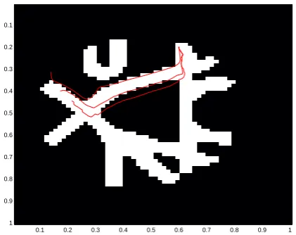
(a) Estimated fibers whenbis 650.
0.1 0.2 0.3 0.4 0.5 0.6 0.7 0.8 0.9 1
0.1 0.2 0.3 0.4 0.5 0.6 0.7 0.8 0.9 1
(b) Estimated curves in (a) with 95% confidence ellipsoids.
0.1 0.2 0.3 0.4 0.5 0.6 0.7 0.8 0.9 1
0.1 0.2 0.3 0.4 0.5 0.6 0.7 0.8 0.9 1
(c) Estimated fibers whenbis 1500 with 95% con-fidence ellipsoids.
0.1 0.2 0.3 0.4 0.5 0.6 0.7 0.8 0.9 1
0.1 0.2 0.3 0.4 0.5 0.6 0.7 0.8 0.9 1
(d) Estimated fibers when b is 2000 with 95% confidence ellipsoids.
Figure 2: Fibers are estimated without clustering tests.
0.1 0.2 0.3 0.4 0.5 0.6 0.7 0.8 0.9 1 0.1 0.2 0.3 0.4 0.5 0.6 0.7 0.8 0.9 1
(a) Fibers are estimated
with-out clustering tests.
0.1 0.2 0.3 0.4 0.5 0.6 0.7 0.8 0.9 1 0.1 0.2 0.3 0.4 0.5 0.6 0.7 0.8 0.9 1
(b) Estimators in (a) with 95%
confidence ellipsoids.
0.1 0.2 0.3 0.4 0.5 0.6 0.7 0.8 0.9 1 0.1 0.2 0.3 0.4 0.5 0.6 0.7 0.8 0.9 1
(c) Fibers are estimated with
clustering tests.
0.1 0.2 0.3 0.4 0.5 0.6 0.7 0.8 0.9 1 0.1
0.2
0.3
0.4
0.5
0.6
0.7
0.8
0.9
1
(a) Tracings of fiber 2 started at different
loca-tions.
0.1 0.2 0.3 0.4 0.5 0.6 0.7 0.8 0.9 1
0.1
0.2
0.3
0.4
0.5
0.6
0.7
0.8
0.9
1
(b) Tracings of fiber 3 started at different
loca-tions.
0.1 0.2 0.3 0.4 0.5 0.6 0.7 0.8 0.9 1
0.1
0.2
0.3
0.4
0.5
0.6
0.7
0.8
0.9
1
(c) Tracings of fiber 5 started at different loca-tions.
0.1 0.2 0.3 0.4 0.5 0.6 0.7 0.8 0.9 1
0.1
0.2
0.3
0.4
0.5
0.6
0.7
0.8
0.9
1
(d) Tracings of fiber 7 started at different loca-tions.