Volume-5 Issue-1
International Journal of Intellectual Advancements
and Research in Engineering Computations
With an efficient time series datasets classification fast accuracy
model for dynamic data sets using classical-k-nn algorithm
1
D. Thiyagarajan,
2N.G.Vaishnave,
3K.Yavanya,
4S.Kalaiyarasi.
Assistant Professor 1, Final year students2, 3, 4 Department of Computer Science and Engineering.
K.S.Rangasamy College of Technology, Tiruchengode, Tamilnadu, India [email protected]
Abstract--Recent years have seen significant
progress in improving both the efficiency and effectiveness of time series classification. However, because of the best solution typically the Fuzzy Nearest Neighbour Algorithm with the relatively expensive Dynamic Time Warping as the distance measure, successful deployments on resource constrained devices remain elusive. Common technique to collect the benefits of Fuzzy Nearest Neighbor Algorithm is without inheriting its time complexity. However, because of the unique property (most) time series data and the centroid typically does not resemble any of the instances, an unintuitive and underappreciated fact. This project shows that it can exploit a recent result to allow meaningful averaging of “warped” times series and this result allows us to create ultra-efficient Nearest “Centroid” classifiers that are at least as accurate as their more lethargic Nearest Neighborcousins.
I.INTRODUCTION
There is increasing acceptance that the Nearest Neighbor (NN) algorithm with Dynamic Time Warping (DTW) as the distance measure is the technique of choice for most time series classification problems. Compare the NN-DTW to nearly all of the most highly cited distance measures in the literature on various datasets and found that no distance measure consistently beats DTW, but DTW almost always outperforms most methods that were
originally touted as superior, based on less complete empirical evaluations.
The nearest centroid classifier is an apparent solution to this problem. It allows us to avail of the strengths of the NN algorithm, while bypassing the latter’s substantial space and time requirements.
Contract Time Series Classification: Given (1) a large time series training dataset, (2) the maximum amount of computation resources available, and (3) as much training time as needed, produce the most accurate classifier possible. Assume that the computational resource constraint will be time, not space, and that it will be given to us in the form of the number of CPU cycles available each second. For ease of exposition assume that the constraint will be given as a positive integer C, which is the number of exemplars per class that can examine when asked to Classify a new object.
Explained in the introduction, based on the consensus of the literature and their own experiments, believe that the best solution will be a variant of Nearest Neighbor classification. While decision trees and Bayesian classifiers are very efficient, the fact that no competitively accurate classifiers for time series based on these methods have been produced in a research area as active and competitive as time series classification, is very effective.
Reducing the data cardinality, and doing NN-DTW on the reduced cardinality data. While classification on suitable reduced cardinality data has little effect on accuracy , it only helps scalability on specialized hardware. Reducing the data dimensionality, and doing NN-DTW on the reduced dimensionality data. This idea has been in the literature for at least two decades, and seems to have been rediscovered many times. The idea works well when the raw data is over sampled.
II.RELATED WORK AND BACKGROUND
The idea that the mean of a set of objects may be more representative than any
individual object from that set dates back at least a century to a famous observation of Francis Galton. Galton noted that the crowd at a county fair accurately guessed the weight of an ox when their individual guesses were averaged [9]. Galton realized that the average
was closer to the ox's true weight than the estimates of most crowd members, and also much closer than any of the separate estimates made by cattle experts.
This idea is frequently exploited in machine learning. For example the Nearest
centroid classifier [10] generalizes the Nearest
neighbor classifier by replacing the set of neighbors with their centroid. It should be noted that there are two separate motivations for using the nearest centroid classifier. Most obviously it is faster, being O(1) rather than O(n). However, and less intuitively, it is also known that some circumstances, the Nearest
centroid classifier is more accurate than the Nearest neighbor classifier (NN)[11].
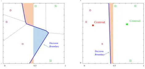
Because it may be counterintuitive that the nearest centroid classifier can be more accurate than NN, we will demonstrate this in an intuitive setting. Consider a domain in which all exemplars are uniformly distributed in the unit square, with objects having an X-value less than 0.5 assigned the label A,
otherwise B. Figure 2 illustrates an example in which there are just three instances per class.
1 1
Centroid Centroid
Decision Boundary
Decision Boundary
0 0
0 0.5 1 0 0.5 1
Figure 2: A simple classification problem in which the concept is the left vs. right side of the unit square. This instance of the
problem has three points per class. left) Here NN has error-rate
of 12.60%, while the Nearest
Centroid classifier (right) with the same instances achieves an error-rate of just 5.22%
It is important to note that the Nearest centroid classifier is not guaranteed to be more accurate than the NN classifier in general.
In spite of the existence of such pathological cases, the Nearest centroid classifier often outperforms the NN algorithm on real datasets, especially if one is willing (as we are) to generalize it slightly; for example, by using clustering to allow a small number of centroids, rather than just one. Thus our claim is simply:
Sometimes NCC and NN can have approximately the same accuracy, in such cases we prefer NCC because it is faster and requires less memory.
Sometimes NCC can be more accurate than NN, in such cases we prefer NCC because of the accuracy gains, and the reduced computational requirements come “for free”.
The difficulty faced by the cognitive scientists is similar to the pragmatic difficulty we face here. In some cases averages may be well defined, for example, the average height of Norwegian man. However, for some objects it is much less clear how to represent and compute averages. For example, computing an average face has been pursued since at least 1883 (again, Francis Galton, using composite photography) but significant progress has only been made in the last decade. Tellingly, this progress in face averaging was exploited to produce dramatic improvements in classification accuracy with a Science paper boasting
Compared to the complexity inherent in faces, time series seem like they would be simple to average, however as Figure 1 hints at, the classic definition of centroid for time series usually produces a prototype which is not typical of the data.
III. DEFINITIONS AND PROBLEM STATEMENT
We present the definitions of key terms that we use in this work. For our problem, each object in the data set is a time series, which may be of different length.
A. Definitions
Definition 1: Time Series. A time series T = (t1, ... ,tL) is an ordered set of real values. The
total number of real values is equal to the length of the time series (L ). A dataset D = {T1, ... , TN} is a collection of N such time
series.
B. Averaging under time warping – related work
Computational biologists have long known that averaging under time warping is a very complex problem, because it directly maps onto a multiple sequence alignment: the “Holy Grail” of computational biology [15]. Finding the multiple alignment of a set of sequences, or its average sequence (often called consensus sequence in biology) is a typical chicken-and-egg problem: knowing the average sequence provides a multiple alignment and vice versa. Finding the solution to the multiple alignment
problem (and thus finding of an average sequence) has been shown to be NP-complete [16] with the exact solution requiring O(LN)
operations for N sequences of length L. Finding the average of a set is best seen as an optimization problem, as explained by the definition below.
Definition 2: Average object. Given a set of objects O = {O1, ... ,ON} in a space E induced
by a measure d, the average object o is the object that minimizes the sum of the squares to the set:
∑
This definition demonstrates that finding the average of a set is intrinsically linked to the measure that is used to compare the data. This means that the average method has to be specifically designed for every measure that is used to compare data.
In our case, the objects are time series and the measure is DTW. We can thus now define what the average sequence should be to be consistent with Dynamic Time Warping.
Definition 3: Average time series for DTW.
Given a set of time series D = {T1,..., TN} in a space induced by Dynamic Time Warping, the average time series ̅ is the time series that minimizes:
∑ ̅
Many attempts at finding an averaging method for DTW have been made since the 1990s. Researchers have exploited the idea that the exact average of two time series can be computed in O(L2). These papers have proposed different tournament schemes (the
guide trees in computational biology) in which the sequences should be averaged first.
(muscle memory) representation of her golf swing or her rendition of a song, of which we can only observe external performance approximations.
C. DBA: the best-so-far method to average time series for Dynamic Time Warping
DTW Barycenter Averaging (DBA), introduced in [8], exploits the parallels between time series and computational biology, while taking account of the unique properties of the former. We have shown in [8] that DBA outperforms all existing averaging techniques on all datasets of the UCR Archive. In particular it always obtained lower residuals (Equation 2) than the state-of-the-art methods, with a typical margin of about 30%, making it the best method to date for time series averaging for DTW.
DBA iteratively refines an average sequence ̅ and follows an expectation-maximization scheme:
1. Consider ̅ fixed and find the best multiple alignment2 of the set of sequences consistently with ̅ .
2. Now consider M fixed and update ̅ as the best average sequence consistent with M . 3. It actually finds the compact multiple alignment.
IV. OBSERVATIONS AND ALGORITHMS Contract algorithms are a special type of anytime algorithms that require the amount of run-time to be determined prior to their activation. In other words, contract algorithms offer a tradeoff between computation time and quality of results, but they are not interruptible.
TABLE I. GENERAL ALGORITHM FOR DBA
Algorithm 1. DBA( D, I )
Require: D: the set of sequences to average
Require: I: the number of iterations 1:
2: 3:
̅= medoid(D ) // get the medoid of the set of sequences D
do times ̅ = DBA_update( ̅,D )
return ̅
Algorithm 2. DBA_update(̅̅̅̅̅̅ ,D )
Require: ̅̅̅̅̅̅ : the average sequence to refine (of
length L)
Require:D: the set of sequences to average 1:
2: 3: 4: 5: 6: 7: 8: 9: 10: 11:
12: 13: 14:
// Step #1: compute the multiple alignment for
alignment = [ ]// array of L empty sets
for each S in D do
alignment_for_S = DTW_multiple_alignment(̅̅̅̅̅̅ , S )
for i=1 to L do
alignment[i] = alignment[i] alignment_for_S[i]
done done
// Step #2: compute the multiple alignment for the alignment
let ̅ be a sequence of length L
for i=1 to L do
̅(i)= mean( alignment[i] )//arithmetic mean on the set
done return ̅
Algorithm 3. DTW_multiple_alignment (Sref , S)
Require: Sref: the sequence for which the alignment is computed
Require: S: the sequence to align to Sref using DTW
1:
2: 3: 4: 5: 6:
7:
8: 9: 10: 11: 12: 13:
// Step #1: compute the accumulated cost matrix of DTW
cost = DTW(Sref , S )
// Step #2: store the elements associated to Sref
L = length(Sref)
alignment = // array of L empty sets
i= rows( cumul_cost ) // i iterates over the elements of Sref
j= columns( cumul_cost ) //j iterates over the elements of S
while (i>1)&&(j>1)do
alignment[i ] = alignment[i ] S(j)
if i--1then j - j - 1
else if j -- 1then i – i – 1
else
14: 15: 16: 17: 18: 19: 20: 21: 22:
cost[i-1][j] )
if score = = cost[i-1][j-1] then
i = i-1 j = j-1
else if score = = cost[i-1][j] then i = i - 1
else j = j-1
end if end if done
return alignment
V.EXPERIMENTAL EVALUATION
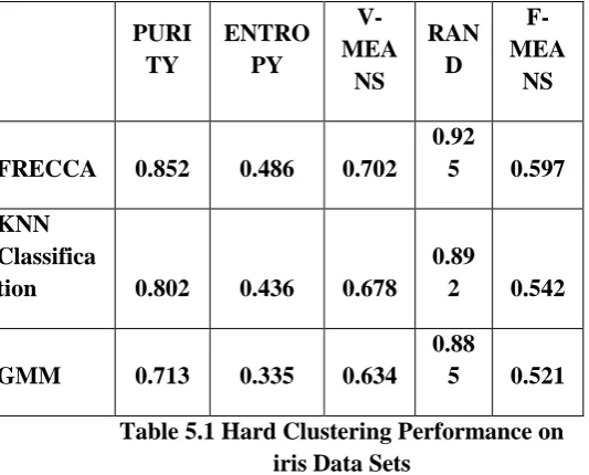
The following Table 6.1 describes experimental result for proposed system analysis. The table contains hard clustering performances for iris data sets in proposed system in purity, entropy, V-mean, Rand and F-Mean details are shown
PURI TY
ENTRO PY
V-MEA
NS
RAN D
F-MEA
NS
FRECCA 0.852 0.486 0.702 0.92
5 0.597
KNN Classifica
tion 0.802 0.436 0.678 0.89
2 0.542
GMM 0.713 0.335 0.634 0.88
5 0.521
Table 5.1 Hard Clustering Performance on iris Data Sets
The following Fig 5.1 describes experimental result for proposed system analysis. The table contains hard clustering performances for iris data sets in proposed system in purity, entropy, V-mean, Rand and F-Mean
The following Table 5.2 describes experimental result for proposed system analysis. The table contains hard clustering performances for heart data sets in proposed system in purity, entropy, V-mean, Rand and F-Mean details are shown
PUR ITY
ENTR OPY
V-ME ANS
RA ND
F-ME ANS
FREC CA
0.93
2 0.533 0.78
2 0.9
65 0.69
7
KNN Classifi
cation
0.93
2 0.526 0.73
8 0.9
62 0.63
7
GMM 0.80
8 0.438 0.78
4 0.9
85 0.66
3
Table 5.2 Hard Clustering Performance on Heart Data Sets
The following Fig 5.2 describes experimental result for proposed system analysis. The table contains hard clustering performances for Heart data sets in proposed system in purity, entropy, V-mean, Rand and F-Mean
The following Table 5.3 describes experimental result for proposed system analysis. The table contains hard clustering performances for additional data sets (data set for iris) in proposed system rand index, NMI (Non-Maskable Interrupt) and F-Mean details are shown
CLUSTER DOC
RAND INDEX
NMI F-MEAN
1 0.500 4.200 0.6608
2 0.342 7.638 0.494
3 0.375 3.557 0.358
4 0.249 7.858 0.329
5 0.334 0.002 0.255
Table 5.3 Proposed Dataset Performances Result
analysis. The table contains hard clustering performances for additional data sets (data set for iris) in proposed system rand index; NMI (Non-Maskable Interrupt) and F-Mean
VI. CONCLUSION
The Dynamic Time Warping (DTW) is able to find the optimal alignment between two time series. It is often used to determine time series similarity, classification and to find corresponding regions between two time series. DTW has a quadratic time and space complexity that limits its use to only small time series data sets. It proves the linear time and space complexity of Fast Accuracy Model The proposed system is having the dynamic time warping and all the averaging techniques that included in the previous system by using different algorithms includes insert, update are also performed with multiple alignment in the existing system space. It also includes the delete operation in the dataset search space in the proposed system space are also included. The dynamic user input for dataset is done in the proposed system. The experimental system shown that clear result on averaging warped time series can be analyzed to allow us to create much faster and are more accurate time series classifiers. The results may be particularly useful for resource constrained situations. The research work improves the search space by expanding the search space by means of implementation with deletion.
SCOPE OF FUTURE ENHANCEMENT
Future work will look into increasing the accuracy of Fast Accuracy Model for DTW using k-NN. Possibilities to increase the accuracy of fast accuracy model for DTW include changing and evaluating search algorithms to guide search during the refinement step rather than simple expanding the search window in both directions.
REFERENCES
[1] X. Wang, A. Mueen, H. Ding, G. Trajcevski, P. Scheuermann, and E. Keogh, “Experimental comparison of representation methods and distance measures for time series data,” Data Mining and Knowledge Discovery, vol. 26, no. 2, pp. 275–309, 2013.
[2] C. Faloutsos, M. Ranganathan, and Y. Manolopoulos. Fast Subsequence Matching in Time-Series Databases. In SIGMOD Conference, 1994.
[3] Jiawei Han and Micheline Kamber. Data Mining: Concepts and Techniques. Morgan Kaufmann Publishers, CA, 2005