Design and DSP Implementation of Fixed-Point Systems
Martin Coors
Institute for Integrated Signal Processing Systems, Aachen University of Technology, 52056 Aachen, Germany Email: [email protected]
Holger Keding
Institute for Integrated Signal Processing Systems, Aachen University of Technology, 52056 Aachen, Germany Email: [email protected]
Olaf L ¨uthje
Institute for Integrated Signal Processing Systems, Aachen University of Technology, 52056 Aachen, Germany Email: [email protected]
Heinrich Meyr
Institute for Integrated Signal Processing Systems, Aachen University of Technology, 52056 Aachen, Germany Email: [email protected]
Received 31 August 2001
This article is an introduction to the FRIDGE design environment which supports the design and DSP implementation of fixed-point digital signal processing systems. We present the tool-supported transformation of signal processing algorithms coded in floating-point ANSI C to a fixed-point representation in SystemC. We introduce the novel approach to control and data flow analysis, which is necessary for the transformation. The design environment enables fast bit-true simulation by mapping the fixed-point algorithm to integral data types of the host machine. A speedup by a factor of 20 to 400 can be achieved compared to C++-library-based bit-true simulation. FRIDGE also provides a direct link to DSP implementation by processor specific C code generation and advanced code optimization.
Keywords and phrases:fixed-point design, design methodology, data flow analysis, compiled simulation, code optimization.
1. INTRODUCTION
Digital system design is characterized by ever-increasing complexity that has to be implemented within reduced time, resulting in minimum costs and short time-to-market. This requires a seamless design flow that allows the execution of the design steps at the highest suitable level of abstraction.
For most digital systems, the design has to result in a fixed-point implementation, either in HW or SW. This is due to the fact that these systems are sensitive to power consumption, chip size, throughput, and price-per-device. Fixed-point realizations outperform floating-point realiza-tions by far with regard to these criteria.
A typical fixed-point design flow is depicted in Figure 1. Algorithm design starts from a floating-point description that is analyzed by means of simulation without taking the quantization effects into account. This abstraction from all implementation effects allows an exploration of the algo-rithm space, for example, the evaluation of different digi-tal receiver structures. This exploration is well supported by
a variety of commercial block-diagram oriented system level design tools [1, 2, 3]. The modeling efficiency on the floating-point level is high and the floating-floating-point models offer a max-imum degree of reusability.
In a next step towards system implementation, a transfor-mation to a bit-true representation of the system is necessary, that is, assigning a fixed word length and a fixed exponent to every operand. This process is quite tedious and error-prone if done manually: often more than 50% of the implementa-tion time is spent on the algorithmic transformaimplementa-tion [4] to the fixed-point level for complex designs once the floating-point model has been specified.
The major reasons for this bottleneck are as follows: (1) There is no unique transformation from floating-point to fixed-floating-point.
(a) Different HW and SW targets put different con-straints on the fixed-point specification.
ok?
Figure1: Fixed-point design process.
Program memory/ chip size
Quantization noise Throughput
Figure2: Fixed-point design space.
space as sketched in Figure 2. Furthermore, targets with a given datapath, for example, DSPs put different constraints on the quantization than ASICs where the datapaths are flex-ible.
(c) The quantization is generally highly dependent on the application, that is, on the applied stimuli.
(2) Quantization is a nonlinear process. Analytical mod-els based on signal theory are only applicable for systems with a low complexity [5]. An exploration of the fixed-point de-sign space with respect to quantization noise, performance, and operand word lengths cannot be done without extensive system simulation.
(3) Some algorithms are difficult to implement in fixed-point due to high signal dynamics or sensitivity to quanti-zation noise. Thus algorithmic alternatives need to be em-ployed.
Finally, the quantized system is implemented, either in hardware or in software on a programmable DSP. The
implementation needs to be optimized with respect to chip area, memory consumption, throughput, and power con-sumption. Here the bit-true system-level model serves as a “golden” reference for the target implementation which yields bit-by-bit the same results.
To increase the designer’s efficiency, software tool sup-port for fixed-point design is necessary. Ideally the design en-vironment would have the following features:
(1) A modeling language supporting generic fixed-point data types to model the fixed-point behavior of the system. It will also provide a means of data monitoring of variables and operands during simulation, for example, range, mean, and variance.
(2) A semiautomatic transformation from floating-point to a bit-true representation. The designer can bring in his knowledge about the system and he has full control over the transformation. The tool will accept a set of constraints spec-ified by the designer to model the characteristics of the target hardware.
(3) The ability to perform bit-true simulation with a sim-ulation speed close to floating-point simsim-ulation.
(4) A seamless design flow down to system implementa-tion, generating optimized input for DSP compilers.
These requirements have been the motivation for the Fixed-point pRogrammIng and Design Environment (FRIDGE) [6, 7, 8], an interactive design environment for the specification, simulation, and implementation of fixed-point systems.
In this article we describe the principles and elements of FRIDGE and outline the seamless design flow as it becomes possible with this design environment. FRIDGE relies on five main concepts which are briefly introduced in the following.
1.1. Fixed-point modeling language
DSP system design is frequently done on a PC or a work-station utilizing a C/C++-based system-level design environ-ment. For efficient modeling of finite word length effects, language extensions implementing generic fixed-point data types are necessary. ANSI C does not offer such data types and hence fixed-point modeling using pure ANSI C becomes a very tedious and error-prone task.
Fixed-point language extensions implemented as li-braries in C++ [9, 10, 11] offer a high modeling efficiency. They supply generic fixed-point data types and various cast-ing modes for overflow and quantization handlcast-ing. The sim-ulation speed of these libraries on the other hand is rather poor. Some of these libraries also offer data monitoring ca-pabilities during simulation time.
In the FRIDGE design environment, the SystemC fixed-point data types are used for fixed-fixed-point modeling and sim-ulation. A more detailed description of the SystemC fixed-point data types is given in Section 3.
1.2. Interpolative transformation
transformation, which is presented in detail in Section 4 uses analytical range propagation to determine operand word lengths.
1.3. Data flow analysis
During the development of the FRIDGE design environ-ment, we have identified a need for accurate data flow anal-ysis. The published approaches for static and dynamic pro-gram analysis did not match the requirements of the de-sign environment, thus we have developed a novel approach for control and data flow analysis, which is presented in Section 5.
1.4. Fast bit-true simulation
Existing C++-based simulation libraries model the fixed-point operands as objects and make extensive use of oper-ator overloading and container data types. Also, for ease of use, many decisions are made during run time. These mecha-nisms increase the execution time of fixed-point simulations by one to two orders of magnitude compared to floating-point arithmetic. This makes the simulation run time a major bottleneck during the fixed-point design process.
In Section 7 various approaches for fixed-point simula-tion are presented and a methodology for fast bit-true sim-ulation by mapping fixed-point algorithms in SystemC to an integer based ANSI C algorithm is introduced.
1.5. DSP target mapping
The final step in a float-to-fixed design flow is the implemen-tation of the DSP system, either in hardware or in software. As a case study for targeting a high performance DSP, we have developed a FRIDGE back end which addresses the Texas In-struments TMS 320C62x fixed-point DSP processor and its C compiler. The back end generates target specific integer C code which exploits the features of the processor and the compiler to achieve a high efficiency of the compiled code. In Section 9 the FRIDGE C62x back end and the optimiza-tion strategies are presented.
2. THE FRIDGE DESIGN FLOW
The FRIDGE design flow starts from a floating-point algo-rithm in ANSI C. As illustrated in Figure 3, the designer then annotatessingleoperands with fixed-point attributes. Insert-ing theselocal annotationsresults in ahybriddescription of the algorithm, that is, some of the operands are specified bit-true, while the rest remain floating-point. A comparative simulation of the floating-point and the hybrid code within the same simulation environment shows whether the local annotations are appropriate, or if some annotations have to be modified. The integer word length of the local annota-tions can be derived from operand range monitoring during simulation runs. Typically, the designer manually annotates function parameters and key variables, for example, accumu-lator variables, which account for approximately 5% of all operands.
Floating-point ANSI-C code
Local
annotations Hybrid code
“Hybrid” simulation
Global annotations
Interpolation
Simulation engine
Fixed-point code
Bit-true simulation
Figure3: Quantization methodology with FRIDGE.
Once the hybrid program matches the design criteria, the remaining floating-point operands are automatically trans-ferred to fixed-point operands by interpolation. Interpola-tion denotes the process of computing the fixed-point pa-rameters of the nonannotated operands from the informa-tion that is inherent to the annotated operands and the op-erations performed on them. Additionally, the interpola-tor has to observe a set of global annotations, that is, de-fault restrictions for the calculation of fixed-point param-eters. This can be, for example, a default maximum word length that corresponds to the register length of the target processor.
The interpolation results in a fully annotated program, where each operand and operation is specified bit-true way. Cosimulating this algorithm with the original floating-point code will give an accuracy evaluation—and for changes now only the set of local and/or global annotations have/has to be modified, while the rest is determined and kept consistent by the interpolator.
Described above are thealgorithmic leveltransformations as illustrated in Figure 1, that change the behavior or accu-racy of an algorithm. The resulting completely bit-true algo-rithm inSystemCis not directly suited for implementation, thus it needs to be mapped to a target, such as, a proces-sor’s architecture or to an ASIC. This is animplementation level transformation, where the bit-true behavior normally remains unchanged. Within the FRIDGE environment, dif-ferent back ends map the internal bit-true specification to different formats/targets, according to the purpose or goal of the quantization process.
3. FIXED-POINT DATA TYPES AND LOCAL ANNOTATIONS
iwl fwl s
wl
wl : word length iwl : integer word length fwl : fractional word length s : sign encoding/sign bit
Figure4: Fixed-point attributes of a bit-true description.
Initiative (OSCI)[11]. Together with additional fixed-point language elements from theA|RT Libraryby Frontier Design Inc., [10]fixed-Chas been the base for the development of the SystemC fixed-point data types that are now used in the FRIDGE project as well.
The SystemC fixed-point data types are utilized for dif-ferent purposes in the FRIDGE design flow:
•Since ANSI C is a subset of SystemC, the additional fixed-point constructs can be used as bit-true annotations to dedicated operands of the original floating-point ANSI C file, resulting in ahybridspecification. This partially fixed-point code can be used for simulation or as input to the interpola-tor.
•The bit-true output of the interpolator is represented in SystemC as well. This allows a maximum transparency of the results to the designer, since the changes to the code are reduced to a minimum and the effects of the designer’s direc-tives, such as local annotations in the hybrid code, become directly visible.
The additional fixed-point types and functions are part of a C++ class library that can be used in any design and simulation environment that are based on or can integrate C or C++ code (see, e.g., [1, 2, 3].)
For a bit-true and implementation independent specifi-cation of a fixed-point operand, a three-tuple is necessary: theword length wl, theinteger word length iwl, and thesign s, as illustrated in Figure 4.
For every fixed-point format, two of the three parameters wl,iwl, andfwl(fractional word length) are independent; the third parameter can always be calculated from the other two, wl=iwl + fwl.
With a given sign encodings, we can also compute the minimum and maximum value that the fixed-point for-mat <wl,iwl>can hold. For example, for a two’s comple-ment (tc) signed representation the minimum and maxi-mum compute to
max wl,iwl,tc=2
iwl−1−2fwl,
min wl,iwl,tc= −2
iwl−1. (1)
For an unsigned representation (us), on the other hand, the minimum and maximum are
max wl,iwl,us=2
iwl−2fwl,
min wl,iwl,us=0.
(2)
Note that anintegraldata type is merely a special case of a fixed-point data type with an iwl that always equals wl— hence an integral data type can be described by two parame-ters only, the word lengthwland the sign encodings.
In the following sections, we provide a short overview of the most frequently used fixed-point data types and func-tions in SystemC. A more detailed description can be found in the SystemC users manual [11].
3.1. The data types sc fixed and sc ufixed
The two’s complement data typesc fixedand the unsigned data typesc ufixedreceive their format when they are de-clared, that is, the fixed-point attributes must be known at compile time (static arguments),
sc_fixed<wl,iwl> d,*e,g[8]; sc_ufixed<wl,iwl> c;
Thus they behave according to these fixed-point parame-ters throughout their lifetime. This concept is called declara-tion time instantiadeclara-tion(DTI). Similar concepts exist in other fixed-point languages as well [9, 10, 15]. Pointers and arrays, as frequently used in ANSI C, are supported as well.
For every assignment to a DTI variable, a data type check is performed. If the left-hand data type does not match the right-hand data type as illustrated in the code example below, an implicit cast to the left-hand data type becomes necessary,
sc fixed<6,3> a,b; sc ufixed<12,12> c;
a = b; /* correct, both types match */ c = b;
/* type mismatch -> implicit cast necessary */
The data typessc fixedandsc ufixed are the data types of choice, for example, for interfaces to other function-alities or for lookup tables, since they behave like a memory location of a specific length and a known embedding/scaling.
3.2. The data type sc fxval
Additionally to the DTI data type concept, SystemC provides theassignment time instantiation(ATI) data typesc fxval. This type may hold fixed-point numbers of arbitrary format and is especially tailored for the float-to-fixed transformation process. A declaration of a variable of typesc fxvaldoes not specify any fixed-point attributes and if subsequently in the code a fixed-point value is assigned to asc fxval vari-able, the variable is (re-)instantiated with all fixed-point at-tributes of the assigned value.
3.3. The data types sc fix and sc ufix
sc fxval cast func(int wl, int iwl, sc fxval in) {
return sc fix(in,wl,iwl);
}
As shown in this example, the constructor for the types sc fixandsc ufixare often used to cast a value to a dif-ferent fixed-point format.
3.4. Cast modes
For a cast operation to a fixed-point format <wl,iwl, sign>, it is also important to specify the overflow and pre-cision reduction in case the target data type cannot hold the original value:
a = sc_fix(input,wl,iwl,q_mode,o_mode);
The variable a holds a two’s complement fixed-point format <wl,iwl> and the value of input is cast to this fixed-point data type according to the quantization mode q mode1 and the overflow mode o mode.2 The most im-portant casting modes are listed below. SystemC also spec-ifies many additional cast modes to model target specific behavior.
Quantization modes
Truncation(SC TRN). The bits below the specified LSB are cut off. This quantization mode is the default for SystemC fixed-point types and will be used if no other value is specified.
Rounding(SC RND). Adds LSB/2 first, before cutting off the bits below the LSB.
Overflow modes
Wrap-around (SC WRAP). In case of an overflow the MSB carry bit is ignored. This overflow mode is the default for SystemC fixed-point types and will be used if no other value is specified.
Saturation(SC SAT). In case the minimum or maximum value is exceeded the result is set to the minimum or maxi-mum value, respectively.
With thesc fxvaltype, every assignment to a variable overwritesall prior instantiations, that is, onesc fxval vari-able may have different context-specific bit-true attributes in the same scope. This concept of ATI is motivated by the spe-cific design flow: transformation starts from a floating-point program, where the designer abstracts from the fixed-point problems and does not think of a variable as finite length reg-ister.
The concept of local annotations and ATI is also an ef-fective way to assign context specific information without changing structures or variables when exploring the fixed-point design space.
1The quantization handling specifies the behavior in case of a word
length reduction at the LSB side.
2The overflow handling specifies the behavior in case of a word length
reduction at the MSB side.
4. INTERPOLATION
The interpolator with its control and data flow analyzer is the core of the FRIDGE design environment. As depicted in Figure 3 it determines the fixed-point formats for all operands of an algorithm, taking as input a user annotated hybrid descriptionof the algorithm and a set of global default rules, theglobal annotationfile. Henceinterpolationdescribes the computation of the fixed-point parameters of the non-annotated operands from the information that is inherent to the annotated operands.
The interpolative concept is based on three key ideas: (1) Attribute propagation. The method of using the at-tributes of the bit-true specified operands in the code to cal-culate bit-true attributes for the remaining operands and op-erations in the code.
(2)Global annotations. The description of default rules and restrictions for attribute propagation.
(3)Designer support. The interpolator supplies feedback and reports to assist the designer to debug or improve the interpolation result.
For a better understanding the first two points are ex-plained more detailed in the following.
(1)Attribute propagation. Given the information of the fixed-point attributes of some operands, the type and the fixed-point format of other operands can be extracted from this information. For example, if for the inputs to an opera-tion both the range and the relevant fracopera-tional word length are specified, the same attributes can be determined for the result.3
Consider the following line of code:
c = a + b; d = 1.5; e = c * d;
The corresponding data flow graph is depicted in Figure 5. We assume that the ranges and the precision of the variablesaandbare known, for example, by user annota-tions:
a∈[−0.25,0.75]=⇒Ra=[−0.25,0.75]; fwl(a)=2, b∈[−1.25,0.5]=⇒Rb=[−1.25,0.5]; fwl(b)=2. (3) To receive the range Rc for the variablecthat contains the sum of the variablesaandbwe add the ranges Raand Rb(a detailed description of the range arithmetic used here can be found in [14]),
Rc=Ra+ Rb=min
a + minb ,maxa + maxb
=[−1.5,1.25]. (4) The precision Pc(fwl) for the sumccomputes to the maxi-mum of the precisions Paand Pb,
Pc=maxPa,Pb=2. (5) The information on the range and on the precision of the variablecis sufficient to calculate the required word length
3An exception is the division, where the accuracy of the operation must
a
[−0.25,0.75]
b
[−1.25,0.5] c
[−1.5,1.25]
d=1.5
e
[−2.25,1.875]
∗
+
Figure5: Example for interpolation of ranges/word lengths.
or integer word length for c. The correlation between fwl, range, and iwl yields the iwl ofc:
iwlc=maxlog2min
c ,log2maxc + 2
−fwlc+ 1
= max(0.58,0.58) + 1=2.
(6)
Thus the resulting format forcis <4,2,tc>, where tc indicates the two’s complement representation of c.
The next step for the interpolator is to compute the fixed-point format of the constantd. Since the range of dis Rd=
[1.5,1.5] and the precision is Pd=fwld=1 the iwl ofdcan be calculated as
iwld=log2max
d +2
−fwl=log
2(1.5 + 0.5)
=1. (7)
After all fixed-point parameters of the input operands to the multiplicatione = d * care known to the interpolator, it continues with the calculation of the bit-true format and parameters for the variablee:
Re=Rc∗Rd=[−1.5,1.25]∗1.5=[−2.25,1.875], Pe=Pc+ Pd=2 + 1=3=⇒iwle
=maxlog2min
e ,log2
max
e + 2
−fwle+ 1
=max(1.17,1) + 1=3.
(8)
Hence we receive a fixed-point format of <6,3,tc>for the variablee.
Note that this is a rather conservative way of interpola-tion, bits that may contain any information are never dis-carded. For the MSB side this is called aworst case interpo-lation, since with the iwl calculated by the interpolator an overflow is impossible, while on the other hand it may lead to iwls much larger than actually needed. In this case the de-signer may add additional local annotations to cut back the iwl to a more suited value. For the LSB side this is called maximum precision interpolation (MPI) interpolation, that is, by default every LSB of the operands is kept, maintaining the highest possible accuracy. LSBs are only discarded if the word length exceeds the maximum word length specified in theglobal annotationfile. This can lead to a large increase in the (fwl), but with additional local annotations the designer can also keep thefwlshorter. In [6] we also describe a method to have the interpolator calculate a less conservative value for thefwl.
(2)Global annotations. While local annotations express fixed-point information for single operands, the global an-notations describe default restrictions to the complete de-sign. For different targets, different global restrictions apply. For SW, the functional units to perform specific operations are already defined by the architecture of the processor. Con-sider a 16×16 bit multiplier writing to a 32-bit register. A global annotation can supply the information to the interpo-lator that the word length of a multiplication operand must not exceed 16 bits, while the result may have a word length of up to 32 bits.
4.1. Implementational issues
In a first step the FRIDGE front end parses in the hybrid de-scription into a C++-based intermediate representation (IR). Then range propagation is performed to determine the bit-true format for all the operands. During this process, control and data flow analysis is also carried out. The information gained is stored in the IR. The advanced algorithms used for the analysis will be described in Section 5.
After this process the IR holds a bit-true description of the algorithm with additional control and data flow infor-mation. These data structures form the basis for additional transformation steps performed in the FRIDGE back ends that target different languages and platforms.
5. ADVANCED DATA FLOW ANALYSIS
During the development of the FRIDGE design environ-ment, we have identified a need for accurate data flow anal-ysis to cater the needs of the interpolation, the fast simula-tion code generasimula-tion and the target specific code optimiza-tion. The published methods were not capable of matching the requirements, thus we have developed a novel approach for data flow analysis that can provide the necessary data for the FRIDGE back ends.
Researchers have worked on program analysis techniques since the 1960s and there is, by now, an extensive literature [16]. There are two major approaches to program analysis:
(a) There are static analysis techniques that analyze the program code at compile time. Usually, sets of equations are set up according to the program semantics and solved by finding their fixpoint. One of the best known static ap-proaches is Data Flow Analysis. It is treated in depth in standard compiler books [17, 18]. Other techniques such as constraint-based analysis and abstract interpretation are also described in [19]. PAG [20] is a tool for generating interprocedural data flow analyzers that implement these techniques.
processed during execution. Thus the results are of no gen-eral nature.
Analysis techniques of neither category are suited for the needs of the FRIDGE design environment. Static anal-ysis puts tight constraints onto the code to be analyzed. The use of pointers is usually not supported or yields too con-servative results. Implementations of digital signal process-ing systems usually make extensive use of pointers, even, for example, for iterating over data arrays. Furthermore, static analysis is blind for program properties that result from run time effects. However, especially these properties have to be taken into account by FRIDGE in order to obtain precise results.
Dynamic analysis is to some extend capable of detect-ing these properties. Nevertheless, it is not applicable for the FRIDGE design environment for two reasons. First, the results are of statistical, numerical nature. There is no way to gain information about data flow or control flow prop-erties. Second, the results are not generally valid, that is, they only reflect the behavior of the program running on the given input vectors. FRIDGE requires analysis results that are valid for all possible executions of the program though.
The requirements for the analysis employed by FRIDGE are different from those of standard tools like, for exam-ple, a general purpose compiler. FRIDGE is focused on digi-tal processing systems. These systems are typically data flow dominated, that is, their execution is to a great extent in-dependent from the data to be processed. Besides, the ac-curacy and quality of the results are more important than speed (of analysis). This allows for a more comprehensive code analysis than, for example, a general purpose com-piler can apply. In order to gain precise results including also run time properties and being able to handle pointer operations, the code is interpreted. Since there is no con-crete data to be processed, we process abstract data instead. In the following this methodology is referred to asabstract execution.
The data flow analysis unit in the FRIDGE design envi-ronment is based on three main components:
(1) The concept of data abstraction. (2) The state controlled memory model. (3) The concept of coupled iterators.
5.1. Data abstraction
While in concrete execution numeric values are written to and read from memory, we useoperationsfor abstract execu-tion. Anoperationis a collection of information about possi-ble values. The two most important elements are
(1) the range, that is, the minimum value and the maxi-mum value, and
(2) a reference to the expression in the code that corre-sponds to the operation.4
4This is for gaining data flow information.
Furthermore, operations may be ambiguous. Consider the code example below.
01 int func(int x, int y, int z){ 02 int a, b, c, d;
03
04 switch(y){
05 case 1:
06 a = 8; break;
07 case 2:
08 a = 16; break;
09 case 3:
10 a = 32;}
11
12 if(z>0)
13 b = 0;
14 else
15 b = 1;
16
17 if(x>0){
18 c = 5;
19 d = a;}
20 else {
21 c = b;
22 d = 7;}
23
24 return c + d; 25 }
The only information available about parametersx,y, andzis that they are integers. Hence it cannot be decided which branches of theswitch- andif-statements in lines 04, 12, and 17 are executed. This results in an ambiguous content, for example, of variable b, namely, values05 and 1, referring to the expressions in lines 13 and 15, respec-tively. We combine both operationsto anambiguous opera-tion. In addition,ambiguous operations are associated with conditions, under which the alternatives are chosen. In the example, alternative 0is chosen if (z > 0)istrue, alter-native1if it isfalse. In general, there may be more than two alternatives and conditions may be combined by a logi-calAND.
Operationsare arranged in graphs similar to binary de-cision diagrams introduced by Akers [23], where the nodes embody the ambiguous operationsand the leafs the unam-biguous operations.
In general, operations are described by the following rules:
(i) anoperationis either anunambiguous operationor an ambiguous operation;
(ii) anunambiguous operationrepresents a possible con-tent in memory during concrete execution of a pro-gram;
5When talking about a value, we mean an operation with a range
Interpreter read/write
State controlled
memory model
Con
tr
o
l
Current state
Me
ss
ag
es
Figure6: Abstract execution.
(iii) an ambiguous operationis associated with a control flow ambiguity in the code (dashed line in Figure 7) and matches each possible branch to anoperation.
Thus these trees do not only contain the alternatives, but also the conditions under which the alternatives are taken. The conditions are determined by all the ambiguities along the path from the root to the alternative. Each ambiguity contributes to the condition in this way, that the condition for the execution of the control flow branch must be fulfilled, that is associated with the link to the nextoperationon the path. A logical AND is applied to the contributions of each ambiguity.
For example, the tree in Figure 7 with A3as its root shows the ambiguity tree corresponding to variable d in line24. The path to value32 (bold line) goes through ambiguities A3 and A4. A3 is associated with theif-statement and the path follows the link that is associated with thetrue-branch. That yields the condition (x > 0) == true. Further on, the path passes through A4and follows the link to 32. A4is associated with theswitch-statement and the link to 32 with case 3. That yields the conditiony == 3. Thus the result-ing condition for A3taking on thevalue32 is6
(x > 0) == true && y == 3
5.2. The state controlled memory model
As illustrated in Figure 6, thestate controlled memory Model serves as a regular memory that can be read and written to. Besides, it is responsible for building the ambiguity trees de-scribed in Section 5.1.
As long as thecurrent stateis in initial state, the behavior of the state controlled memory model does not differ from a regular memory. Once thecurrent statecontains a condi-tion, all changes done to memory contents only occur un-der that condition and result in appropriate ambiguity trees. The state is defined by a set of assumptions about the re-sult of particular expressions in the code. A logical AND is performed on these assumptions. The initial state makes no assumptions at all. Other valid states could for example be “(x > 0) == true” or “(x > 0) == true && y == 3.” During abstract execution, the state can be changed by the interpreter.
6This notation is according to C syntax.
if (x >0)
A1
true 5 false true
A2
false 0
1
if (z >0)
switch (y)
A3
true false
A4
7
case 1: 8 case 2:
16 case 3:
32
Step
Nr. Currentstate
(1)
(2)
(3)
(4)
(5)
(6)
(x >0)==t&&y==1
(x >0)==t&&y==2
(x >0)==t&&y==3
(x >0)==f&&(z >0)==t
(x >0)==f&&(z >0)==f
Figure7: Iterating over ambiguities.
5.3. Iterating over ambiguities
When abstractly executing statements (Section 5.4) or com-puting the set of all possible evaluations of an expression,7 We have to iterate over the alternatives of ambiguities. This is basically done by traversing the corresponding tree. However, thecurrent stateis taken into account, that is, only those alter-natives arevisible, whose conditions are not contradictory to thecurrent state. Furthermore, when selecting an alternative from an ambiguity, the corresponding conditions are—if not yet included—added to thecurrent state. This way, the fol-lowing is achieved: All data couplings are taken into account, that is, no impossible cases are considered. Alternative exe-cutions of statements can be done without further thought about thecurrent state(see Section 5.4).
Selecting an alternative from an ambiguity is done by building a path through the corresponding tree. The end of the path is anunambiguous operation. In principle, iterating
7For example, this is done when computing fixed-point parameters of an
is performed on all successors of an ambiguity first, until it will be iterated over the alternatives of the ambiguity itself (depth first). When establishing a path through an ambigu-ity, two basic cases have to be considered:
(1) Thecurrent statecontains a condition respective to the control flow fork that is associated with the ambiguity. In this case, the pathmustfollow the link that corresponds to the condition and may not be altered. The node would be considered aslavenode.
(2) Thecurrent statedoes not yet contain a condition re-spective to the control flow branch that is associated with the ambiguity. In this case, a possible branch is selected and the path is extended by the corresponding link. The correspond-ing condition is added to thecurrent state. The node would be considered amasternode. During further iteration, the path will switch to all other links successively. When this is done, the respective condition has to be updated accordingly. After that, the condition is removed from thecurrent state.
The trees in Figure 7 show the contents of variables c (left-hand side) and d (right-hand side) connected to line 24in the code. Figure 7 also illustrates how to iterate over all possible combinations of contents of both variables. Note how building a path through an ambiguity affects the cur-rent stateand how thecurrent statemasks the visible alter-natives of ambiguities. First of all value5 is selected from ambiguity A1. The corresponding condition ((x > 0) == true) is added to thecurrent state. Thus A1becomes a mas-ter node. When building the path through A3, A3 becomes a slave node, because thecurrent statealready makes an as-sumption about the control flow ambiguity that is associated with A3((x > 0)). Therefore, the pathmustfollow the link from A3to A4. Nodes A2and A4are associated with different control flow forks, respectively. They always become master nodes and never affect any other ambiguities. Steps 2 and 3 it-erate over the remaining visible alternatives of the right-hand tree. Step 4 switches to the second alternative of master node A1(false). This affects the slave A3in this way as long as the path in the left-hand tree goes from A1to A2(steps 4 and 5), the only visible alternative of the right-hand tree is7. In step 6 the iteration has been completed.
5.4. Execution of a program
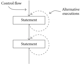
Figure 8 shows how statements are abstractly executed. The solid lines represent the control flow of a concrete execu-tion. Abstract execution also follows that control flow. How-ever, statements that depend on ambiguous data are executed multiple times (dashed lines), once for every possible vector of the involved ambiguities. The vectors are iterated over as described in Section 5.3. Thus every execution is performed in a differentcurrent state, such that changes in memory to-gether with their corresponding states are stored in ambi-guity trees. This algorithm is applied recursively for nested statements. Any code constructs can be executed this way.
Although a possibly large number of execution states ex-ists, we found that the run time and the memory consump-tion of the analysis were remarkably low for typical signal processing algorithms. In most cases the control and data
Control flow
Statement
Statement
Alternative executions
Figure8: Abstract executions of sequential statements.
flow analysis was performed in less than one second on a 800 MHz PC.
The information gained during abstract execution is stored in the intermediate representation of the algorithm. The FRIDGE back ends, which will be introduced in the next sections, access this information to perform several code transformation steps.
6. FAST BIT-TRUE SIMULATION
As pointed out in Section 1, transforming a signal processing algorithm from a floating-point to a fixed-point requires ex-tensive simulations due to the nonlinear nature of the quanti-zation process. The available C++-based fixed-point libraries [10, 11] offer a high modeling efficiency but the simulation speed of these libraries on the other hand is rather poor. This makes simulation speed a major bottleneck in the fixed-point design process.
Utilizing C-based fixed-point libraries like the ETSI ba-sic arithmetic operations [24] does not overcome this prob-lem as the simulation speed still has a considerable overhead compared to an equivalent floating-point implementation.
Existing C++-based simulation libraries model the fixed-point operands as objects. In order to offer generic fixed-point data types without word length restrictions, data con-tainer types are used as an internal representation. Bit-true operations are performed by operator overloading. Range checking, the choice of cast modes and many other decisions necessary for correct bit-true behavior are done at simula-tion time. The price for this flexibility and ease of modeling is slow execution speed as the generic fixed-point data types modeled by extensive C++ constructs cannot be efficiently mapped to the architecture of the host machine by today’s C++ compilers.
Another mean of speeding up fixed-point simulations is the use of a hardware accelerator, for example, an FPGA to perform computationally expensive operations. The acceler-ation can be achieved either by utilizing configurable logic or by combining configurable logic with a processor. This ap-proach has been described by De Coster [26]. The mapping of the algorithm to the different hardware units and the data transfer between the units make additional transformation steps necessary.
The work described in this article proposes a mapping of fixed-point algorithm in SystemC to an integer-based ANSI C algorithm that directly addresses the built-in integer ALU of the host machine. An efficient mapping includes an em-bedding of all fixed-point operands into the host machine registers, a cast mode optimization and many other aspects, and requires a detailed control and data flow analysis of the algorithm. Independently from the authors’ work, De Coster [26] proposed a similar method, using DFL [27] as input lan-guage and targeting directly a Motorola DSP65000.
Our work presented here represents a continuation of the research results published by Keding et al. [6] and Willems [14] and introduces improved concepts for the mapping pro-cess that result in a considerable simulation acceleration.
For the fast simulation back end we assume that fixed-point attributes are assigned to every operation. The back end also requires the information collected during the con-trol and data flow analysis stored in the IR. After a number of IR refinements, an ANSI C representation of the algorithm using only integral data types can be derived from the IR. It is important to note that the transformation in the back end, in contrast to the float-to-fixed transformation in the IR, does not change the behavior of the algorithm. The fully quantized algorithm coded inSystemCand the integer-only ANSI C algorithm yield bit-by-bit identical results, making the fast simulation back end output ideally suited for fast bit-true simulation on a workstation or PC.
7. TRANSFORMATION TO ANSI C
7.1. The lbp alignment
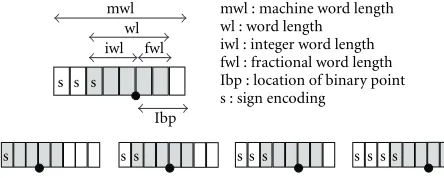
For the embedding of a fixed-point operand specified by a triple(wl, iwl, sign)into a register of the host machine with the machine word length (mwl) the minimum requirement is
mwl≥wl=iwl + fwl. (9) Figure 9 illustrates different options for embedding an operand with a word length of 5 bit into a given mwl of 8. Obviously, for mwl >wl, a degree of freedom for choosing the location of binary point (lbp) exists:
mwl−iwl≥lbp≥wl−iwl=fwl. (10) Beside this degree of freedom, there are also a number of constraints for the selection of the lbp:
(i)Interface constraints. For interface elements, such as, function parameters or global variables, the lbp must be
de-mwl wl iwl fwl
s s s s s s s s s s
Ibp s s s
mwl : machine word length wl : word length
iwl : integer word length fwl : fractional word length Ibp : location of binary point s : sign encoding
Figure9: Embedding a 5-bit word into an 8-bit register.
fined identically for a function and all calls to this function. Otherwise, the data written to or read from these data ele-ments will be misinterpreted.
(ii)Operation constraints. Each operation has an lbp syn-tax. This lbpsyntaxmay include constraints on the lbp of the operand(s) of the operation and/or rules for the calculation of the lbp of the result. For example, the operands and the result of and addition must have the same lbp.
(iii)Control and data flow constraints. Generally, a read access to a storage element must use the same lbp as the pre-ceding write access to the storage element. This implies that if a write operation to a memory location occurs in alternative control-flow branches, the lbp must be at the same position in both write operations, as no run time information about the lbp is available in a following read operation. The same applies to ambiguous write operations to arrays and write operations via pointers.
7.1.1 The lbp alignment algorithm
The lbp alignment algorithm implemented in the fast sim-ulation back end is designed to take advantage of the de-gree of freedom described by (10), while meeting the con-straints specified above. Meeting these concon-straints and main-taining the consistency of the lbps require precise informa-tion about the control and data flow of the algorithm. To ob-tain this information we used the data flow analysis method described in Section 5. The data flow information is repre-sented basically asdefine-use (du) chainsanduse-define (ud) chains[17, 18], with additional and more accurate informa-tion about ambiguous control flow.
Initially, for all operands lbp = fwl is chosen. Thus all operands areright aligned. In a first step we set the lbps of all interface elements according to theinterface constraints.
Then, in an iterative process, the data flow information is used to adjust the lbps by insertion of shift operations to meet theoperation constraintsand thecontrol and data flow constraints. The algorithm terminates when all conditions are fulfilled and the lbps did not change during the last iteration. The operation constraint lbp alignment algorithm basi-cally consists of an iteration over all operations and an ad-justment of the operand and result lbps according to the op-eration’s lbpsyntax.
(ud-chains). According to the control and data flow constraints the lbp of operands linked by such ud-chains are set to the same value.
Finally, the embedding ofconstantscan be done in a way that the required shift operations when using the constant are minimized.
Unlike described by Kum et al. [28], we do not use a shift operation minimizing approach here, but using the degree of freedom in choosing a suited lbp (10) and the accurate data flow information, we found that there is not sufficient potential for this optimization to justify the effort.
7.2. Data type selection
The next step in the transformation process is the selection of suitable integral data types for fixed-point variables. The FRIDGE internal bit-true specification of the algorithm fea-tures arbitrary word lengths. With the SystemC back end this does not represent a problem, since the SystemC data types are generic and may be of any bit length required. With the fast-simulation back end, on the other hand, we only have the limited pool of the built-in data types of the host machine, that is, integral data types likechar,short,int,long.
7.2.1 Basic constraints for any data element
A matching data type for every fixed-point variable has to be chosen. The minimum requirement for the data type chosen is that it can be embedded into the host machine data type with word length mwl at the correct location, (see Figure 9 for illustration) iwl + lbp≤mwl.
7.2.2 Structural constraints
Additionally, the requirements introduced by data structures that force each of their elements to be of the same data type have to be met. An example for this behavior are arrays. The target data type for theNelements of an array must fulfill the following condition: maxN−1
i=0 (iwlarray[i] + lbparray[i])≤mwl. 7.2.3 Semantical constraints
Another constraint becomes important if aliasing of data el-ements, for example, by pointers occurs: a pointer may point to different data elements. For syntax and semantics reasons all aliased data elements and the base type of the pointer must be identical [13]. This only causes a problem if data types are changed like it is done in fixed-point optimizations or the floating-point to fixed-point transformation process de-scribed in Section 2: initially, most numerical data types are floating-point types but after the transformation there are various different fixed-point data formats. Hence special care must be taken during the code generation process to ensure that the types are consistent. A detailed description of the data type selection algorithm used can be found in [29].
7.3. Cast mode transformation
Cast operations can reduce or limit the word length on the MSB side of a word (overflow handling) or at the LSB side of a word (quantization handling). They are used either to
pre-vent indeterministic behavior of fixed-point systems8 or to model a data path that is different from the host machine. This is often the case when algorithms for DSP systems are developed. Fixed-point libraries like in SystemC offer various generic overflow and quantization handling modes, which makes SystemC an efficient means of modeling fixed-point systems. For fast fixed-point simulation, on the other hand, the use of these generic casting modes are simply ruled out for performance reasons.
7.3.1 Overflow handling
Overflow handling is required if it is necessary to reduce the wl at the MSB side of the word or if the carry bit is set for the MSB. Examples for frequently used overflow handling modes in digital signal processing algorithms arewrap-aroundand saturation[30].
Saturation
In SystemC, a cast of an expressionexprto awl-bit tc data type with integer word lengthiwlapplying saturation as over-flow mode can be modeled as follows:
result = sc_fix(expr,wl,iwl,...,SC_SAT);
The fast simulation code generation on the other hand trans-lates this into plain C code that first tests if the range of data type is exceeded, and if so it sets the resulting value to the minimum or maximum of this type, which is
MAX wl,iwl,lbp,tc=2
iwl+lbp−1−2lbl−fwl, MIN
wl,iwl,lbp,tc= −2
iwl+lbp−1+ 2lbl−fwl−1. (11)
Thus the fast simulation code construct generated is the fol-lowing:9
int tmp;
result=((tmp=expr)>MAX)?MAX:(tmp<MIN)?MIN:tmp;
Introducing an additional temporary variable avoids multi-ple evaluations ofexpr.
Wrap-Around
The SystemC way of casting an expressionexprto awl-bit tc data type with integer word lengthiwlapplying wrap-around as overflow mode is shown here,
result = sc_fix(expr,wl,iwl,...,SC_WRAP);
For the bit-true ANSI C equivalent of this operation sev-eral options exist. An example for a code construct forwrap around assuming two’s complement arithmetic and a ma-chine word length of mwl is
8In many cases, the ANSI C standard [13] does not specify the bit-true
behavior of integral data types in case of overflow, quantization, and so forth.
9Note that for the code generation we also take the bit-true properties of
result = (expr << SHIFT) >> SHIFT;
The amount of shifts computes to SHIFT=mwl−iwl− lpb. The shift left eliminates the MSBs whereas the arithmetic shift right provides a sign extension for the new MSB.
7.3.2 Quantization handling
If the word length of an operand is reduced at the LSB side, we can apply different quantization handling modes. The most frequently encountered areroundingandtruncation.
Rounding
In SystemC the method for casting an expressionexprto a wl-bit two’s complement data type with integer word length iwlapplying rounding as quantization mode is
result = sc_fix(expr,wl,iwl,SC_RND,...);
Rounding is defined by adding DELTA = LSB/2 to the operand and eliminating the LSBs, for example, by shifting it right SHIFT=lbp−fwl bits. Thus the rounding operation can be realized in the fast simulation code by
result = ((expr + DELTA)>>SHIFT)<<SHIFT;
Truncation
The truncation operation, given in SystemC by
result = sc_fix(expr,wl,iwl,SC_TRN,...);
can be implemented efficiently by a bit mask operation,
result = expr & (~MASK);
Where MASK is given by 2lpb−fwl−1.
For several combinations of cast modes, for example, wrap-around combined with rounding or truncation, more efficient joint quantization and overflow handling C code constructs are generated. The shift operations introduced by the cast code constructs are also utilized to adjust the lbp of the expression, eliminating the need for additional scaling shifts.
8. EXPERIMENTAL RESULTS
The code generated by the FRIDGE fast simulation back end has been benchmarked against the fixed-point simula-tion classes, which are part of the C++-basedSystemC lan-guage. The simulation classes offer two simulation modes: a mode supporting unlimited fixed-point word lengths based on concatenated data containers and a mode supporting lim-ited precision up to 53 bits based on float-arithmetic and bit manipulations.
The benchmarks have been performed on a SUN Ul-tra 10 workstation running SOLARIS using the GCC com-piler version 2.95.2 with the -O3option. The SystemC li-brary version 1.0 was utilized for the bit-true simulations. The benchmark is based on typical signal processing ker-nels,FIR17-tap FIR filter,DCT8×8 JPEG DCT algorithm,
Autocorr 25 elements 5th order autocorrelation, IIR 3rd order IIR filter,FFTcomplex FFT of length 8,Matrix4×4 matrix multiplication.
Four different versions of the kernel functions have been benchmarked:
(i)Floating-Point.The execution speed of the floating-point implementation of the algorithms serve as reference for the benchmarks.
(ii)SystemC.The quantized bit-true version of the algo-rithms utilizing theSystemCfixed-point data types. The al-gorithms have been quantized using theFRIDGEdesign en-vironment.
(iii) SystemC limited precision. The quantized bit-true code has been compiled with thelimited precision optionto speed upSystemCfixed-point operations.
(iv)Fast simulation code.The fast fixed-point simulation code based on integral data types has been generated by the FRIDGE back end applying the transformation techniques described in the previous sections. The code yields bit-by-bit the same results as the code utilizing theSystemCdata types. The experimental results are presented in Table 1. As the floating-point code has been used as a reference, the exper-imental data has been scaled relative to the execution speed of the floating-point code. The bit-true SystemCcode con-sumes by a factor of 325 to 1103 more run time than the orig-inal floating-point code, making bit-true simulation a major bottleneck in the fixed-point design flow. Utilizing the lim-ited precision mode of theSystemClibrary, a speedup by a factor of 3.1· · ·5.2 can be achieved, but the fixed-point code is still by a factor of 67· · ·234 slower than the floating-point reference.
The fast simulation code runs by a factor of 18.8· · ·90.9 faster compared to the SystemC fixed-point code utilizing thelimited precisionoption. For theunlimited precisionthe speedup is 91.0· · ·454.2, respectively.
Compared to the floating-point reference code, the fast simulation code is by a factor of 2.5· · ·6.9 slower. This is due to the host system’s architecture and additional shift and bit mask operations necessary to perform lbp-alignment and cast operations to maintain bit-by-bit consistency with the quantized code.
The quantized DCT algorithm contains many cast oper-ations to reduce fixed-point word lengths introduced by the quantization process. As these operations can be modeled ef-ficiently by bit mask operations in the fast simulation code, the highest speedup was achieved for this kernel function.
9. DSP CODE GENERATION
de-Table1: Relative execution speed.
Floating-point ANSI C SystemC SystemC limited precision Fast simulation code
FIR 1.0 386.5 102.7 2.8
DCT 1.0 1103.1 233.9 2.5
Autocorr 1.0 694.6 130.6 6.9
IIR 1.0 371.0 120.2 3.1
FFT 1.0 354.7 67.7 2.6
Matrix 1.0 325.9 71.2 3.6
veloped using a processor/compiler codesign methodology which led to compiler-efficient processor designs.
On the other hand, a significant gap in the system design flow is still evident; there is no direct path from a floating-point system level simulation to an optimized fixed-floating-point implementation. Today a manual implementation on the DSP and target specific code optimization is necessary, in-creasing time-to-market and making design changes very te-dious, error prone, and costly. Thus we have developed an optimizing FRIDGE back end to generate target optimized DSP C code. The target specific code generation is necessary for two reasons:
(i) The generic point data types used for fixed-point simulations are not suited for DSP implementation, as the currently available DSP compilers do not support C++ fixed-point data types. The upcoming generation of DSP compilers will support C++ language constructs, but com-piling the fixed-point libraries for the DSP is no viable al-ternative as the implementation of the generic data types makes extensive use of operator overloading, templates, and dynamic memory management. This will render fixed-point operations rather inefficient compared to integer arithmetic performed on a DSP.
(ii) Compiling the FRIDGE-generated integer ANSI C code on a DSP is also not sufficiently efficient as the generic C code does not exploit the capabilities of the DSP hardware such as built-in saturation and rounding logic or SIMD pro-cessing.
As a case study, we have chosen the TMS320C62x pro-cessor and its C compiler as a target for the FRIDGE de-sign environment.This enables a seamless dede-sign-flow from floating-point to optimized C62x C code utilizing integral data types. Generating a C62x optimized version of a signal processing algorithm using a different set of fixed-point pa-rameters becomes a matter of hours instead of days or weeks using the conventional manual techniques. The C62x integer code generated by the design environment yields bit-by-bit the same results as the fixed-point code utilizing C++ simu-lation classes on the host machine. Thus a comparative sim-ulation to the “golden reference model” gives the designer a high degree of confidence in the generated code.
The first objective of our case study was to find out which C code constructs compile into efficient C62x as-sembly code. Thus we applied the DSPstone benchmarking methodology to the C62x optimizing C compiler. The DSP-stone project [31], conducted in 1994 by ISS, Aachen
Uni-versity of Technology established a benchmarking method-ology for DSP compilers by comparing the performance of compiled C code to hand optimized assembly code in terms of program/data memory consumption and execution time. As a consequence, it allows to identify a possible mismatch between architecture and compiler. The benchmarking has been done using eleven typical signal processing algorithms (FIR, FFT, DCT, minimum error search, etc.). The bench-marking gives quantitative results for cycle count and pro-gram memory consumption.
In a second step, we used C62x specific C language ex-tensions (intrinsics) and compiler directives to restructure the off-the-shelf C code while maintaining functional equiv-alence to the original code. These optimizations led to a con-siderable improvement in performance in many cases as the compiler was able to utilize software pipelining and instruc-tion level parallelism to speed up the code. It has turned out that software pipelining is the key to achieving a high per-formance but, on the other hand, requires careful analysis and code restructuring. The evaluation [32] gave quantita-tive performance data for the C62x compiler and a set of code optimization techniques to generate efficient C62x C code.
In a third step, we benchmarked various implementa-tions of the fixed-point quantization and overflow handling modes on the C62x. This led to a set of optimized implemen-tations for the quantization and overflow handling function-ality.
9.1. DSP code transformation
The FRIDGE C62x back end performs similar transforma-tion steps as the fast bit-true simulatransforma-tion code generatransforma-tion presented in Section 6: lbp alignment, cast mode transfor-mation, and data type selection. Additionally, target specific code optimization is performed.
The designer has to keep the special requirements of the DSP target in mind to reach a high level of efficiency. Through our experiments we found that, for example, the number of cast statements and shift operations has a strong influence on the efficiency of the generated code. Thus if the designer chooses settings for theglobal annotationsand the default cast modeduring the early stages of the transforma-tion which do not represent the properties of the target ar-chitecture properly, the code optimization and the DSP com-piler are not able to generate efficient assembly code.
com-piler with the best C code possible. The amount of analy-sis done in an optimizing compiler is usually limited due to constraints of the time used for compilation. In the FRIDGE design environment, control and data flow analysis is per-formed with the maximum possible accuracy utilizing the techniques presented in Section 5. The information gained during this analysis is available for the back end code trans-formation as well. Thus we are able to perform code restruc-turing techniques, which are usually beyond the scope of an optimizing compiler.
9.1.1 The lbp alignment
As the TI C6000 processor family has aninteger multiplica-tion mode, theright alignmentstrategy of the lbp alignment algorithm can also be applied in the C62x back end. This al-gorithm implicitly minimizes the number of scaling shifts. In contrast to the fast bit-true simulation, the number of scal-ing shifts generated is important for the C62x code genera-tion. For the fast simulation code generation we found the potential of shift minimization limited to a performance im-provement of 3%· · ·13% [29]. This is different for the C62x code generation. As the C62x can perform two scaling shift operations per cycle, a shortage of functional units limits the performance in highly software pipelined loops. Thus “shift poisoning” of loops must be avoided, for example, by choos-ing suitable fixed-point data types for function parameters and central data structures.
9.1.2 Data type selection
As the properties of the data paths of the C62x processor and the width of the integral data types supported by the C62x C compiler are known, the design environment can utilize this information during the transformation process. A set of global annotations for the C62x guides the interpolation pro-cess and a set of integral data types with a given bit length is supplied to the C62x back end.
9.1.3 Cast mode transformation
The generic overflow- and quantization handling modes of-fered by SystemC have to be mapped to the target hardware in an efficient manner. The C62x offers built-in saturation hardware which can be used by the back end. This is illus-trated by the following example.
Cast mode: saturation
A cast of an expression to awl-bit two’s complement data type with integer word lengthiwlapplying saturation as over-flow mode is modeled in SystemC as follows:
result=sc_fix(expr,wl,iwl,...,SC_SAT);
An implementation of this code construct in generic ANSI C is
int tmp;
result=((tmp=expr)>MAX)?MAX:(tmp<MIN)?MIN:tmp;
On the C62x thesshlintrinsic (saturating shift left) can be used to perform the saturation operation:
result=(signed)_sshl(expr,SHIFT)>>SHIFT;
where SHIFT is given by mwl−(iwl+lbp). Utilizing the built-in saturation hardware of the C62x via thesshlintrinsic al-lows the generation of code with linear control flow in con-trast to the forked control flow in the ANSI C implementa-tion. This significantly speeds up the code.
9.1.4 Loop optimizations
The key to high execution speed on the C62x is software pipelining and instruction level parallelism. This is especially important for loops, where most of the execution time is spent for most digital signal processing algorithms. The latest version of the C62x C compiler is able to perform quite so-phisticated loop optimizations to achieve high performance. This can be further improved by restructuring the loops at source level, applying techniques like loop unrolling, scalar expansion and splitting data paths. By introducing SIMD (single instruction multiple data) intrinsics it is possible to reduce the required number of load/store operations signif-icantly. The C62x back end utilizes the data- and control flow information and the code transformation infrastructure to identify possible loop optimizations and to perform the necessary loop restructuring. The design environment main-tains the consistency of generated code.
10. EXPERIMENTAL RESULTS
We have benchmarked the cycle count performance of the generated C62x integer C code using two sets of typical sig-nal processing kernel functions: The first set consists of six off-the-shelf kernels which have been initially coded with-out DSP specific code optimization. The second set of kernels has been extracted from TI’s C6000 compiler benchmarking suite.
10.1. Off-the-shelf kernels
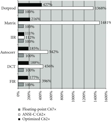
This set of kernels consists of six signal processing functions, which also have been used for the benchmarks in Section 8: FIR, DCT, Autocorr, IIR, Matrix, Dotprod. The code has been translated using TI’s C6x compiler version 4.0 [33] and the performance has been compared with three reference codes:
(i)C67x floating-point C code.The C67x floating-point DSP is code-compatible to the C62x and its C compiler is mostly identical to the C62x C compiler, thus the perfor-mance of the generated fixed-point C code can be compared to the original floating-point C code.
(ii) C62x floating-point emulation. The floating-point emulation library which is part of the C62x compiler’s run time library allows the user to perform floating-point arith-metic on the C62x processor. The floating-point operations are executed as function calls.
Table2: Cycle count.
Floating-point Float emulation Generic ANSI C Target specific C
Device C67x C62x C62x C62x
FIR 132 1304 523 234
DCT 331 34163 1509 622
Autocorr 564 6581 3057 1041
IIR 73 708 82 81
Matrix 108 4999 1600 233
Dotprod 95 9436 1300 406
0%
200% 400% 600% 800% 1000% 1200% 1400% 1600%
Floating-point C67×
ANSI-C C62×
Optimized C62×
Dotprod
Matrix
IIR
Autocorr
DCT
FIR
427%
1368% 100%
216%
1481% 100%
111% 112% 100% 185%
542% 100%
188% 456% 100%
177% 396% 100%
Figure10: Cycle count relative to floating-point code.
Table 2 presents the benchmarking results for the six ker-nel functions. Figure 10 illustrates the relative cycle count. As the C67x floating-point code has been used as a reference, it was scaled to 100%. For readability the results of the floating-point emulation have been omitted in the bar graph.
As depicted in Table 2 the C62x floating-point software emulation has a cycle count which is by a factor of 9.7 to 103 higher than the cycle count of the same code compiled for the floating-point processor.
The generic ANSI C integer code without C62x specific language extensions is by a factor of 1.1 to 14.8 slower than the floating-point code. The integer code performs addi-tional shift- and masking operations to ensure the bit-true behavior. Some of the cast-operations cannot easily be modeled in generic ANSI C. Thus a significant overhead is introduced for kernel functions where many cast operations are inserted by the interpolation (e.g., the DCT).
The performance can be improved by matching the gen-erated code to the target architecture. For example, utilizing the sshl intrinsic is a convenient way to access the C62x
sat-uration hardware directly. This reduces the overhead intro-duced by the additional shift and cast operations to a factor of 1.1 to 4.3 compared to the floating-point code.
For the floating-point code of theDotprodkernel func-tion, the compiler was able to generate efficient code using 95 cycles for 64 vector elements. For the fixed-point code, the additional operations needed for cast operations in the inner loop prevent the compiler from achieving similar efficiency. Removing all scaling shifts and overflow protection from the inner loop of the fixed-point code for this kernel yields a cy-cle count of 83. Introducing a single scaling shift in the inner loop brings the cycle count up to 147, adding overflow pro-tection yields 406 cycles. Similar effects appear in theMatrix kernel benchmark.
10.2. TI compiler benchmarking kernels
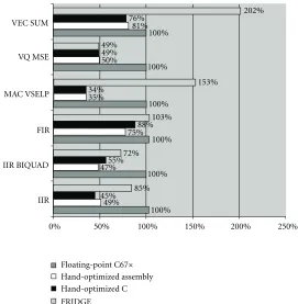
This set of kernels consists of six signal processing functions: IIR16-coefficient IIR filter,IIR cas biquads10 cascaded bi-quads,FIR10-tap 40 sample FIR filter,MAC VSELPtwo 40 samples vectors,VQ MSEMSE between two 256 element vec-tors,VEC SUMvector sum of two 44 sample vectors.
For these kernels hand-optimized C62x assembly code and C62x integer C code is available on TI’s website. It is noteworthy that neither the C code nor the assembly code was coded with overflow protection. For the embedding of input and output operands, implicit assumptions were made which reduced the number of scaling shifts in the kernel functions. Thus the hand-optimized C62x assembly code can serve as an “upper bound” for the efficiency of the FRIDGE C62x design flow.
We derived the floating-point code from the integer C code. The function interfaces in the floating-point code were manually annotated with fixed-point specifications to get hy-brid code. The hyhy-brid code was used as input to generate op-timized C62x integer code from the FRIDGE C62x environ-ment. The FRIDGE generated C62x code features full over-flow protection and maintains consistency for the “location of binary point” for input and output operands. The code has been translated using TI’s C6x compiler version 4.0 [33] and the performance has been compared to the reference codes:
(i)C67x floating-point C code.This is the floating-point code compiled for the C67x processor.
Table3: Cycle count.
Floating-point Assembly Hand optimized ANSI C FRIDGE
Device C67x C62x C62x C62x
IIR 85 42 38 72
IIR BIQUAD 149 70 82 108
FIR 315 237 278 373
MAC VSELP 175 61 59 207
VQ MSE 559 279 275 275
VEC SUM 63 48 51 127
0% 50% 100% 150% 200% 250%
Floating-point C67×
Hand-optimized assembly Hand-optimized C FRIDGE VEC SUM
VQ MSE
MAC VSELP
FIR
IIR BIQUAD
IIR
202% 76%
81% 100% 49%
49% 50%
100%
153% 34%
35%
100% 103% 88% 75%
100% 72% 55% 47%
100% 85% 45%
49%
100%
Figure11: Cycle count relative to floating point code.
(iii) C62x hand-optimized assembly code. The hand-optimized assembly code served as a reference for the bench-marks.
Table 3 presents the benchmarking results for the six ker-nel functions. Figure 11 illustrates the relative cycle count. For consistency, the floating-point code has been used as a reference, it was scaled to 100%.
For these kernels, the C6x compiler was obviously able to generate very efficient code. For consistency we have mea-sured the cycle count including the function call. This causes the optimized C code to be faster than the hand-optimized assembly code for some kernels. The floating-point code is slower than the hand-optimized assembly and C code in all cases as the floating-point instructions need more execution stages than their integer counterparts. For