Paper 04-2019-1

A Proposed Damping Coefficient of Quick Adaptive Galerkin

Finite

Volume Solver for Elasticity Problems

S. R. S. Yazdi1_{, T. Amiri}2*_{, S. A. Gharebaghi}3

1_{Civil Engineering Faculty, K. N. Toosi University of Technology, Tehran, Iran}

[email protected]

2_{Civil Engineering Faculty, Sirjan University of Technologhy, Sirjan, Iran}

[email protected]

3_{Civil Engineering Faculty, K. N. Toosi University of Technology, Tehran, Iran}

[email protected]

*corresponding author

Abstract

A Quick Adaptive Galerkin Finite Volume (QAGFV) solution of Cauchy momentum equations for plane elastic problems is presented in this research. A new damping coefficient is introduced to preserve the efficiency of the iterative pseudo-explicit solution procedure. It is shown that the numerical oscillations are not only effectively damped by the proposed damping coefficient, but also that the rate of the convergence of QAGFV algorithm increases. Furthermore, the numerical results show that the proposed coefficient is not sensitive to the spatial discretization. In order to improve the accuracy of the computed stress and displacement fields, an automatic two-dimensional h–adaptive mesh refinement procedure is adopted for shape-function-free solution of the governing equations. For verification, two classical problems and their analytical solutions have been investigated. The first is a uniaxial loaded plate with holes, and the second is a cantilever beam under a concentrated load. The results show a good agreement between QAGFV and analytical method. Moreover, the direct and iterative approaches of the finite element method have been implemented in FORTRAN to evaluate the efficiency and accuracy of the presented algorithm. In the end, the corresponding results of some problems have been compared to the QAGFV solutions. The results confirm that the presented h-adaptive QAGFV solver is accurate and highly efficient especially in a large computational domain.

Keywords: Galerkin Finite Volume Method, Numerical Damping Relation, A Posteriori Error Estimator, h–Adaptive Mesh Refinement, Unstructured Triangular Meshes

1. Introduction

The Finite Volume Method (FVM) is usually a second–order accurate numerical approximation, based on the integral form of the governing equations. This method uses a segregated solution procedure, where the coupling and nonlinearity are treated in an iterative way. The method leads to diagonally dominant matrices, which are well suited for iterative solvers (Jasak & Weller 2000c).

Similar to aforementioned methods, the Finite Difference Method (FDM) needs a mesh to discretize the computational domain. Although using the unstructured meshes for dealing with irregular boundaries provides great flexibility in modeling real-world problems (Sabbagh–Yazdi and Alimohammadi 2009), FDM suffers from numerical errors and inefficiencies for solving boundary value problems on irregular domains. As a result, this is a potential bottleneck to handle complex geometries in multiple dimensions by FDM. This issue motivates researchers to use the integral form of the governing equations, which results in FEM and FVM (Yip 2005).

Here, there is a compromise between high expenses of FEM direct solver for large matrices or cheaper expenses of FVM iterative solver. Owing to the fact that FVM is inherently good at treating complicated, coupled and nonlinear differential equations, it is widely used in fluid flows. In recent years, computational fluid dynamics has been dealing with high order meshes that are necessary to produce accurate results of complex mathematical models and full–size geometries (Jasak and Weller 2000c). When a mathematical model becomes more complex, FVM becomes more interesting alternative compared to FEM. In addition, unlike FDM, FVM solution is conservative in which the incompressibility is exactly performed for each control volume of computational domain (Alkhamis et al. 2008). Due to local conservation properties, FVM should be in a good position to effectively solve structural analysis of linear, non-linear and incompressible materials. Moreover, FVM numerical calculation on meshes consisting of triangular cells showed excellent agreement with the analytical results (Sabbagh–Yazdi and Alimohammadi 2009).

Ekhteraei–Toussi et al. demonstrated that FVM offers some advantages over the equivalent FEM models. Their results show the local and global norms of numerical errors for FVM are similar to FEM and similar stiffness matrix is created using the constant strain triangular elements. Therefore, the results’ accuracy is comparable in both methods. Interestingly, the execution time for FVM is less than direct FEM for a fine mesh (Ekhteraei–Toussi and Rezaei–Farimani 2007). Although FVM was originally developed for computational fluid dynamics, some problems in continuum mechanics have been successfully resolved using this method (Demirdžić and Martinović 1993).

nonlinear problems (Boroomand and Zienkiewicz 1999). Li and Wiberg (1994) used h–adaptive Finite Element Analysis (FEA) to more accurately simulate 2D linear elastic structural problems on meshes consisting of triangular cells. Later, it was extended to quadrilateral meshes (Sharif and Wiberg 2002). Katragadda and Grosse performed a FEA to investigate the influence of the dual loading (thermal and static) on quadrilateral meshes using the h–adaptive scheme. They modified the Zienkiewicz and Zhu (𝑍𝑍2_{) technique to improve the convergence and}

computational efficiency (Katragadda and Grosse 1996). Tabarraei et al. developed an h–adaptive FEM using quad–tree data structure and polygonal interpolants for better efficiency. Adaptive FEM is nonconforming on quad–tree mesh; therefore, Tabarraei and Sukumar (2005) used mesh– free basis function to construct conforming approximation. Phongthanapanich and Dechaumphai (2004) employed the Delaunay triangulation as the mesh generator. They predicted the crack propagation path for practical problems of mechanical engineering. Meyer et al. (2006) numerically simulated the crack propagation of linear elastic problems. They used 2D adaptive solver on triangular meshes to obtain more accurate solution and used the hierarchical data structure to improve the efficiency of analysis. This data structure would not be destroyed during crack propagation analysis, therefore the efficiency of the analysis increases. Khoei et al. (2008) used the automatic adaptive re-meshing procedure for the numerical simulation of crack growth in the context of FEM. They used the 𝑍𝑍2 _{error estimator with the modified SPR technique using}

the analytical solution at the crack tip to obtain more accurate error estimation. Palani et al. (2006) proposed a new error estimator based on either Strain Energy Release Rate (SERR) or Stress Intensity Factor (SIF). They used the proposed error estimator at the crack tip region. For regions away from the crack tip, the residual error estimator based on stress was used. They performed the fracture analysis of 2D problems on quadrilateral meshes using the proposed method. The SPR method was developed to transfer data of 3D elasto–plasticity problems during adaptive FEA by Gharehbaghi and Khoei (2008). They used the polynomial function with C₀, C₁ and C₂ continuity to estimate required values of state variables and error (Gharehbaghi and Khoei 2008). Afshar et al. (2012) used the adaptive refinement procedure to solve the elasticity problems using the least squares concept and the Meshless Method. They presented residual a posteriori error estimator to detect the regions of high error.

problems on triangular meshes. They utilized residual a posteriori error estimation in the adaptive refinement procedure.

Considering the abovementioned efforts, it may be concluded that most researches focused on the adaptive technique in the context of FVM, which has been developed for fluid mechanics problems. Thus, adaptive FVM in solid mechanics could be a novel strategy.

The presented numerical solution may introduce spurious oscillations, which is related to pseudo-explicit time integration of Galerkin Finite Volume Method (GFVM) formulations. These oscillations could smear the numerical solution, and consequently may result in the loss of accuracy. In this research, a new damping coefficient relation is firstly introduced to damp the unwanted oscillations of the pseudo-explicit solution of Cauchy equations to preserve the efficiency of the iterative pseudo-explicit procedure. The GFVM solution results show that this relation increases the rate of the convergence and effectively damps the numerical oscillations. Later, the effects of mesh refinement on the proposed damping coefficient are studied. The obtained numerical results show that the proposed coefficient is not sensitive to the spatial discretization. In addition, the effects of the introduced coefficient on the accuracy of the numerical results are also studied.

As already mentioned, the large scaled and complicated problems include calculation of the large stiffness matrix using FEM. Bearing in mind that solving simultaneous equations directly is expensive in such problems and leads to very high computational cost and low efficiency, this research presents a fast, efficient and accurate matrix free FV algorithm, which gives high-precision results at a very low computational cost. In this research, the QAGFVA implemented in FORTRAN is used to solve the PDEs governing stress–strain fields. In addition, both direct and iterative FEMs are implemented in FORTRAN to evaluate the efficiency and robustness of the presented FV technique. The 2D automatic adaptive procedure is used for more accurate simulation of the plane elasticity problems using GFVM and FEM. Finally, an error estimator is used to discover the regions of high error, then the mesh refinement is performed to increase computational accuracy. The accuracy and efficiency of the presented method are evaluated by comparing the computational results of displacement and stress with the analytical solutions and numerical results of others.

In the first section, Cauchy equations, the governing equations of solid mechanics, are briefly described. The discretized form of Cauchy momentum equation is derived using GFVM in section 2.1. Further on, the new damping coefficient relation is introduced to damp the undesirable numerical oscillations, associated with pseudo-explicit solution of Cauchy equations. In section 3, the equilibrium equation and Generalized Minimum Residual Method (GMRES) are described in Finite Element framework. Consequently, the error estimation analysis and h-adaptive method are presented. Ultimately, the numerical examples are provided to validate the proposed model.

2. Galerkin finite volume method

2.1. Plane–elasticity equations

The Cauchy momentum equation is a PDE, which can be derived by applying the Newton's second law to a control volume in a continuum. This equation can be expressed in Equation (1) as the governing equation of solid mechanics.

ij f fVir V_t

σ ρ∂

∇ + + =

Where ρ and V are the material mass density and velocity, respectively. σij and f are the stress

tensor and body force. f_Vir = −CV is the viscous damping force, which is added to eliminate the numerical oscillations resulted from the quasi-explicit solution of the system of equations. C is the damping coefficient kg₃

m s

     .

For 2D problems in x y− coordinate system, the stress tensor is presented as following:

T

xx yy xy

σ _{= }σ σ σ _ (2)

The compatibility relations for strain-displacement are:

xx yy xy u x v y u v y x ε ε ε  _∂    ∂        ∂  =    _∂        ∂ ∂  +   ∂ ∂   (3)

The stress–strain relation is expressed as:

11 12

21 22

33

xx yy

xx

yy xx yy

xy xy D D D D D ε ε σ σ ε ε σ γ    +      = +             (4)

Which for plane–stress is defined as follow:

(

)

₍

₎

11 12 13

21 22 23 ₂

31 32 33

1 0 1 0 1 1 0 0 2

D D D v

E

D D D D v

v

D D D v

      _{ }   =_{ }=   − _{ }   ₋   _{ }     (5)

2.2. Galerkin finite volume formulation

GFVM discretizes the Cauchy momentum equation using the Galerkin method and integrating over the domain. In this method, a suitable weight function φ is selected. The weight function should be integrable and its values on the boundaries of the corresponding node, Γ, is equal to zero. Now, both sides of the Cauchy equation are multiplied by the weight function, and the resulted equation is integrated over the domain as Equation (6):

( )

( )

. ij . . .

Vir

n n

j n n

V

d f d f d d

x t σ φ φ φ φ ρ Ω Ω Ω Ω ∂  _{Ω + Ω + Ω =}  ∂  _Ω   _{ } _∂  _{ ∂ }  

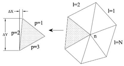
Fig. 1. Control Volume of node "𝑛𝑛" with triangular elements

The weight function φ could be chosen as the linear shape function of the triangular element. Therefore, for a constant-strain triangular element, the weight function equals to 1 in the node “n” and 0 in the other nodes of the control volume (Figure 1).

By defining Li =σi1i+σi2j

 

, the first term of the left hand side of the Equation (6) can be expressed as:

( )

(

)

. ij . . | .

i _n i i

n n

j _n

d L d L L d

x σ φ φ φ _Γ φ Ω Ω Ω ∂  Ω = ∇ Ω = − ∇ Ω   _∂   

∫

∫

∫

(7)

The first term in the right hand side of the above equation is eliminated due to the zero value of the weighting function on Γ. Moreover, the second term in the right hand side of the Equation (7), which includes the spatial derivatives, can be rewritten as follows:

(

)

3

(

)

1 1

. .

2

i i

n _l l

L φ d L l

= Ω

∇ Ω ≈ −

∑

∆

∫

(8)

In which

( )

∆l ₁ is the normal vector of boundary edge 1 from the nth Ω_n sub-domain. In addition, FDM is used to discretize the time-dependent term on the right hand side of Equation (6). In order to simplify the remaining terms of Equation (6), the following equation is used:

( )

( )

.

3n

nd n

φ χ χ Ω Ω   Ω ≈ _{ }  

∫

(9)

In which χ is the body force or viscous damping force. Finally, the discretized form of the Cauchy momentum equation in the ith direction is rewritten as follows:

( )

(

( )

)

(

)

( ) ( )

( )

( ) ( )

(

)

1 2 1 1 1

3 _{. 2 , 1,2}

2

k k

N _S k

k k _{n n n} k k

i

i n n i _l k i n i n

l

n _n

u u

C f

u t F l u u i

t ρ ρ ρ − + − =   ₋     = ∆ ∆ + − + − =   Ω  _ ∆ _ 

∑

 (10)

In which,

( )

u k_n+1 is the displacement of the node “n” in the𝑖𝑖th direction at iteration

(

k+1

)

. Ω_n

is the area of the control volume, and N is the number of boundary edges of Ω control volume. The time step

( )

∆t in Equation (10), has no physical interpretation. In fact, it is just a virtual parameter, which has been used to converge the iterative solution.

3 11 12 1 3 12 11 1 3 22 22 1 1 1 1 x y l l n xx x y yy _l l n xy x y l l n

D u y D u x A

D u y D u x A

D u y D u x A σ σ σ = = =  _{ }  ∆ + ∆  _{ }            = ∆ + ∆    _{ }           ∆ + ∆        

∑

∑

∑

(11)

In which, An is the area of the triangular element (Sigma notation is applied on three sides of an

element) (Figure 1). The stress values are computed in the center of the triangular elements.

2.3. Proposed damping coefficient

The C_n parameter in Equation (10) is a damping coefficient used to damp the undesirable oscillations. Here, the damping coefficient relation is introduced to filter the numerical oscillations associated with matrix–free GFVM solution.

The ideal linear viscous damper has been adopted as a dissipative method in the present research. The damping coefficient,

(

[ ]

C =α

[ ] [ ]

K +β M

)

, is computed by calculating the stiffness and mass matrices and estimating α and β. These parameters have arbitrary values. However, they should be large enough to eliminate the spurious oscillations and small enough not to leave negative impact on the accuracy of the results. The calibration of these parameters is necessary to obtain the accurate numerical results. In this paper, NASIR* (Sabbagh–Yazdi 2016) solver, which performs stress analysis using GFVM on unstructured meshes, is used. Since the implemented numerical method is a matrix-free technique, the damping coefficient matrix calculated using the above equation is not suitable to use in NASIR. Therefore, a relation of the damping coefficient is introduced in Equation (12) that could be easily implemented in NASIR solver. This relation quickly eliminates the numerical oscillations associated with pseudo–explicit GFVM solution of the Cauchy momentum equations.

( )

2 3/ |1 | *

n

C = E− −Vol n E ρ (12)

In Equation (12), Vol n( ), ,ρ E are the area of the control volume, the material mass density and Young’s modulus, respectively. Equation (12) automatically estimates the correct damping coefficient of structural problems for pseudo–explicit matrix–free GFVM procedure regardless of α and β parameters. In addition, Equation (12) is independent of mass and stiffness matrices. Fast computation and convenient implementation in the applied numerical code are the other merits of the proposed damping coefficient.

In order to verify the proposed numerical damping, the external load is applied using three different ways. The first way is called Length Scale, which gradually applies the given load. The second way is Sudden Loading, which suddenly applies the load without the numerical damping. The last one is called Numerical Damping, which suddenly applies a given load and uses the proposed damping coefficient. The results presented in Section 5 confirm that the numerical oscillations are effectively damped using the proposed damping coefficient. Besides, this coefficient increases the rate of the convergence of the QAGFVA algorithm. Moreover, the numerical results show that the proposed coefficient is not sensitive to the spatial discretization.

3. Finite element method

3.1. Equilibrium equations

Solid mechanics problems could be formulated in terms of minimizing the potential energy function Π as Equation (13):

1

1 _{, 0}

2 T T b T s T i

i i

V V S

dv f f p

ε σ δ δ δ

δ

=

∂Π

Π = − − − =

∂

∑

∫

∫

∫

(13)

Finally, the equilibrium equations could be rewritten in a matrix form as follows:

[ ]{ } { }

K u = F (14)

Where

[ ] { }

K , u and

{ }

F are the global stiffness matrix, displacement vector and load vector, respectively. More details about the Finite Element techniques are provided in Reddy and Gartling (2010).

Equation (14)(14) indicates a system of simultaneous linear equations. There are two main types of methods for solving systems of linear equations: (1) direct methods, in the sense that they converge to the exact solution in a finite number of steps; and (2) iterative solution methods, which present an approximate solution to the system of equations.

Gaussian elimination algorithm is a well-known method for solving simultaneous linear equations. The Gaussian elimination method requires _{2 / 3n}3 _{+O n}

( )

2 _{operations, and n}2_+n storage amounts for solving a system of n linear equations, presented in Equation (14). This method reduces the coefficient matrix to the identity matrix. Thus, it can be quite expensive if n is large (Reddy and Gartling 2010).

Because of round-off errors, the direct methods have less efficiency than iterative methods when they are applied to large system of equations. In addition, the amount of storage space required for iterative solutions is much less than the direct methods. As a result, iterative methods are more attractive than direct methods, especially for sparse matrices.

The iterative methods are classified in different groups such as the basic iterative methods (splitting methods, Jacobi, Gauss-Seidel, Successive over Relaxation (SOR)), the Chebyshev iterative method, the Krylov subspace methods (Conjugate Gradient Method (CGM), Generalized Minimal Residual (GMRES), etc.). The GMRES method is widely used for solving very large and non-symmetric linear systems. Therefore, the authors decided to use it for the iterative FEA.

3.2. The generalized minimal residual (GMRES) method

GMRES method can be used for both symmetric and non-symmetric systems. It generates a sequence of orthogonal vectors for symmetric systems. However, in the absence of symmetry this can no longer be done with short recurrences; instead, all calculated vectors should be saved. The common form of GMRES is based on a modified Gram-Schmidt orthonormalization procedure and uses restarts to control storage requirements.

Note that the system of linear equations

(

F Ku=

)

with matrix K and vector F can be solved by GMRES. This method approximates the exact solution by un∈Kn that minimizes the norm

n n n

u =Q y (15)

Where u_n is the approximation of the solution at the next iteration and y_n minimizes the norm of the residual and all vectors q_i form all columns of Q_n matrix

The Hessenberg matrix

( )

_H_{n is derived from the Arnoldi process as following:}

 1 n

n n

KQ =Q H+ (16)

Therefore:



1

2 n

n n

Ku −F = H y −γe (17)

where:

(

)

1 1,0,0,0,...,0 , 0

T

e = γ = F Ku− (18)

Where u₀ is the first trial vector. Finally vector u_n can be found by minimizing the norm of the residual

( )

rn as Equation (19):



1

n

n n

r =H y −γe (19)

This process is repeated if the residual rn is not yet small enough (Kelley 1995).

4. Adaptive strategy

The solution of most problems is partially uniform in the computational domain, but local phenomena such as strong discontinuity destroy monotonicity. Thus, uniform meshes are not a desired choice to solve governing PDEs. In other words, using large elements will lead to unacceptable results in regions experiencing aforementioned phenomena, but using small elements throughout the computational domain will increase the computational efforts without significant improvement in some regions of the domain (Tabarraei and Sukumar 2005). Therefore, to obtain more accurate Finite Element solution, either more accurate shape functions must be used or meshes must be refined in the regions of high error.

Various adaptive strategies have been produced which are: 1) h–refinement which tends to refine the size of elements; 2) p–refinement, which uses more accurate shape function by increasing the order of polynomials of approximation; 3) r–refinement in which the location of computational nodes are modified; 4) hp–refinement, which refines the size of elements and increases the order of shape functions; 5) hpr–refinement, which is combination of the abovementioned procedures (Palani et al. 2006).

Gosman 2003). Owing to the fact that all adaptive strategies need the value of error to improve the mesh, so a proper error estimator plays a significant role.

4.1. Error estimation analysis

Three main sources of errors are round-off error, convergence error and discretization error. When the real numbers are shown by a finite number of digits, the round-off errors are common. The numerical solution requires an iterative process. The convergence error are due to improper truncation criteria of iterative process (Versteeg and Malalasekera 2007). The discretization error is attributed to the modeling of the computational model with limited degrees of freedom (DOF) instead of the continuum. In addition, the governing equations could be satisfied only in weak sense and in a global point of view. Besides, the boundary conditions are also not fulfilled in an exact manner (Palani et al. 2006). The error estimated in this section belongs to discretization errors.

A posteriori error estimator is required to investigate the analysis accuracy of problems with unknown exact solution and as a stopping criterion in the adaptive procedure (Flaherty 2005). It is recommended that a good error estimator has all the following properties: 1) the error is given in terms of absolute values, 2) it represents reliable information about the error distribution, 3) it can be easily calculated, based on the last solution, 4) it also works well on coarse meshes, 5) it can be used for all forms of the equations., 6) it slightly overestimates the actual error (Jasak and Gosman 2000a). Many studies have focused on error estimation which most researches could be classified into 5 categories: 1) residual based methods (Jasak and Gosman 2003), 2) post– processing methods (Jasak and Gosman 2003), 3) duality methods (Jasak and Gosman 2003), 4) solution of local problem (Bank and Weiser 1985), and 5) hierarchical basis error estimation (Bank and Smith 1993). The first two methods are used more than the others. For more details about the error estimation techniques in FEM, the reader is referred to (Zienkiewicz and Zhu 1987; Zienkiewicz and Taylor 2000; Palani et al. 2006).

The error estimators in FVM are still under development in comparison with FEM. Richardson extrapolation is an error estimator, which is widely used in FVM. It needs two solutions on two different meshes (Jasak and Gosman 2003). There are good references about the error estimation techniques of FVM (Ilinca et al. 2000; Jasak and Gosman 2003).

This research is focused on the post–processing adaptive technique of the Galerkin Finite Volume Method. In fact, the error is identified as the difference between the numerical solution and the corresponding recovered result. In addition, Babuška et al. showed that the post–processing methods are accurate and robust and these methods provide more accurate error estimation than the residual based methods (Zienkiewicz et al. 1999).

In the present study, the displacement of the node “n” in ith direction at iteration

(

k+1 ,

) ( )

u_{i n}k+1, and the element stress, 1

n

k ij

σ + _{, are numerical solution. For convenience, the above-mentioned}

variables are denoted as

(

ui,σij

)

. The corresponding computational errors may be presented as

follows:

,

Ex Ex

u i i s ij ij

e =u −u e =σ −σ (20)

In which, Ex i

u and Ex ij

σ are the exact values. Since there is no information about the exact solution of the problem, the recovered solution

(

*_, *

)

i ij

* _, *

u i i s ij ij

e ≅u u− e ≅σ −σ (21)

The difference between the corresponding values, given in Equation (21), represents the point wise errors of the displacement and stress and the point wise errors are difficult to compute. The estimated error, based on the integration process, could be used as Equation (22) which provides error estimation in a global point of view (Palani et al. 2006).

1/2

T

s s

e e De d

Ω

 

=_ Ω_



∫

 (22)

Where D is the constitutive matrix. The above equation takes into account the contribution of all elements (Equation (23)) and represents the global norm of error.

( )

(

)

( )

( )

1 2

2 2

2 2 2

11 21 22 33

1 1

2

Ncel Ncel

x i x y y xy i

i i i i

i i

e e dS D dS dS D dS D dS D d

= =

 _{ } 

= =_{ } + ∗ + + _ Ω _

 

 

∑

∑

(23)

Where: * * * x x x

y y y

xy i xy xy

dS dS dS σ σ σ σ σ σ     −     = −        ₋       (24)

Where Ncel represents the total number of elements in the computational domain and e_i is the element error norm. The matrix D For plane-stress problems has been presented in Equation (5) and for plane–strain problems, D is represented as following:

(

)

(

)(

)

(

)

(

)

11 12 13

21 22 23

31 32 33

1 0

1

1 0

1 1 2

1 2

0 0

2

D D D

E

D D D D

D D D

υ υ υ υ υ υ υ υ    −    _{ } −   =_{ }= _{+ −}  −      ₋   _{ }     (25)

After computing the global norm of error and the local element error norm, the permissible error norm for each element could be computed considering the target percentage error η_Aim, and total number of elements as:

( )

Aim i i Aim

e e

Ncel η ∗

= (26)

Thus, the new size of each element is given by Equation (27), in such a way that the desired percentage error is achieved (Zienkiewicz and Zhu 1987).

(

) (

)

( )

*

1 ,

old i i

new i i

i Aim i e H H e φ ψ χ χ

= = (27)

Where φ is the minimum of the two orders: (1) the intensity of singularity; and (2) the order of shape function. ψ is considered to be equal to 1

In the present paper, the Superconvergent Patch Recovery (SPR) technique is used to compute the recovered solution. According to SPR technique, the recovered stress field is assumed to be a continuous polynomial expansion with unknown coefficients.

(

)

*

0 2 ... n ,

ij ix y ny F x y

σ =α +α +α + +α = α (28)

Where F x y

(

,

)

is the vector of polynomial terms and α is a vector, which contains all the unknown coefficients. The unknown coefficients could be obtained by minimizing the norm of the difference between the new field and the approximate solution as follows:

(

)

(

)

{

}

2

1

, ,

0

K K ij K K

k

i

F x y x y

ζ

α σ

α

=

 

∂_ − _

 _{ =}

∂

∑

(29)

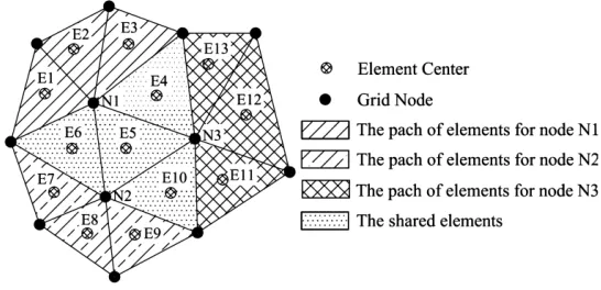
Where ζ represents the number of sampling points. To recover the stress at a given node, all elements, which are common to the node, are found. In fact, a patch of elements is constructed to recover the stress at each given node. The patches for nodes N1, N2 and N3 could be seen in Figure 2. In the next step, according to the location of sampling point in a constant-strain triangular element, the value of stress in each element is assigned to the central (sampling) point of that element. Consequently, the SPR technique is applied to the patch, and the best polynomial is fitted to the stress values of sampling points. Finally, the value of recovered stress is computed in grid nodes. The recovery phase is performed for all stress components of all grid nodes. Then value of stress in each element is computed by fitting the recovered stress at its nodes.

Fig.2. The element patch for fitting procedure

4.2. h–refinement

At the first stage of the analysis, the computational domain is discretized into a coarse but uniform triangular mesh, using an automatic 2Dunstructured mesh generator. In this stage, Delaunay triangulation technique (Thompson et al. 1999) may be applied to the domain. One of the key steps in the implementation of the adaptive re-meshing technique is new mesh generation, which is based on the approximate solution. More precisely, according to the errors of the first analysis, which is performed using the uniform mesh, the new size of each element in all regions of the solution domain is computed. Later, a new mesh is regenerated using this data.

4.3. Data transfer operator

relative error. Subsequently, a new non-uniform mesh is generated using the new element sizes, which are computed by Equation (27). It is clear that the new mesh uses fine elements in the regions of high error and coarse elements in other regions. It is a good idea to continue the analysis with the new mesh to avoid restarting all previous computations. To achieve more performance, it is required to transfer the solution history of the old mesh to the new mesh. In such case, all variables must be transferred to the new mesh during the adaptive procedure (Jasak and Gosman 2000b).

So far, several methods have been proposed by different researchers to transfer computational data between two meshes. Because the transferred variables have not been derived from the new mesh and some incompatibilities may appear. For example, the transferred stress field may not match with the applied loads. Thus, it is better to transfer fewer variables between two meshes. In this study, just the displacement field is transferred from the old mesh to new one. Consequently, the stress–strain field is achieved by the stress analysis on the new mesh using the transferred displacements.

In the first step of the procedure of data transfer, each grid node of the new mesh is searched within the old mesh. For node “N” of the new mesh, the triangular element in the old mesh, which contains the node, is found. Then, the displacement field at node “N” of the new mesh is obtained by fitting the nodal displacements of the old element using the least square manner (Figure 3).

Fig.3. The patch of elements

5. Verification of the developed adaptive algorithm

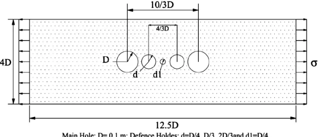
5.1. Uniaxial loaded plate with holes

Adaptive Galerkin Finite Volume Analysis (QAGFVA). The mechanical properties used in the QAGFVA are provided in Table 1.

Fig.4. Schematic illustration of plate with main and defense holes

Mechanical Properties Value (Unit)

Elasticity Modulus E=200 GPa

Density 7854 kg₃

m ρ=

Poisson's ratio v=0.3

Stress σ =10000

Table 1. Mechanical properties of specimen

Due to the symmetry, only one quarter of the plate is considered as the computational domain and the symmetric boundary condition are used on the edges in the symmetry planes to simulate the full plate. The initial mesh is shown in Figure 5. As can be seen, the linear triangular elements are used to discretize the computational domain.

Fig.5. Initial unstructured meshes for adaptive Finite Volume analysis

The initial mesh is adapted during the adaptive analysis, and finally the optimal mesh is achieved considering a target relative error of five percent. The refined mesh for 2

3

Fig.6. The refined mesh for 𝑑𝑑= 2𝐷𝐷�₃

The stress concentration factor, computed across the width of plate, are compared to the published FEA results (Meguid 1986). Computational results across the width of plate for the main and larger defense hole are presented in Figure 7, which shows the high precision of the QAGFVA. From Figure 7, it could be observed that the classic Finite Volume Analysis uses coarse elements in high stress concentration regions and causes less accurate numerical results, while QAGFVA provides more precious results.

Fig.7. Variation of stress concentration factor across the plate width (a) the Main hole; (b) the Defense hole

Fig.8. Maximum principal stress contours computed by the developed model

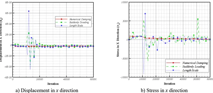
Figure 8 shows the contour of the maximum of principle stress for 2 3

d= D. Figure 9 presents the converged displacement and stress in x directions at an optional node with coordinates (0.2105, 0.0830). If a body with negligible physical damping is suddenly subjected to an external load, computational difficulties due to lack of numerical diffusion may happen. Thus, the gradual load imposing technique was adopted in the previous studies (Sabbagh–Yazdi and Amiri– SaadatAbadi 2013). Although this technique could prevent the oscillations, it needs more iterations to impose completely loading for equilibrium cases. As a remedy, in this research the damping coefficient has been presented to overcome numerical difficulties. According to the following figures, the best convergence rate is seen in the curve of Numerical Damping. The relative error between the numerical values of stress and displacement and the theoretical values is fully damped after few iterations using this damping coefficient.

Fig.9. The convergence of the computed numerical results at an optional node

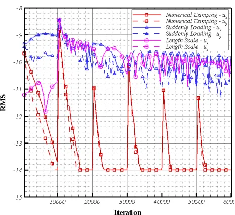
To provide a better understanding of the effects of gradual load imposing technique and the efficiency of the proposed damping coefficient, the convergence of the logarithm of root mean square of the computed displacement in x,y direction, which is calculated by Equation (30), is shown in Figure 10 for three FVM computational models and corresponding loading strategies.

(

1

)

1 log

N

k k

i i _j

j

u u

RMS

N

+ =

 

−

 

 

= _{ }

 

 

 

∑

(30)

Where

( )

k

i _j

u and N are the displacement of _jth _{node in k}th _{iteration, in direction i and the}

Fig.10. The convergence history of the logarithm of root mean square of the displacements in x,y direction

In order to evaluate the efficiency of the presented Adaptive Finite Volume technique, direct Finite Element and GMRES Methods were developed in FORTRAN. The required computational time, which is needed by Central Processing Unit (CPU) to perform the analyses, is considered as a performance criterion. The CPU times of adaptive analysis for three above-mentioned methods are given in Table 2. As can be seen, the present model has a very high performance, compared to the direct Finite Element. Besides, QAGFVA overcomes the GMRES, according to CPU time criterion.

Method Number of _Nodes Number of _Elements CPU Time _(Second) Adaptive Finite Volume Analysis

(QAGFVA) 1691 3164 4.53

Adaptive Finite Element Analysis (AFEA)

Direct 1598 3105 85.14

Iterative

(GMRES) 1587 3097 7.31

Table 2. The comparison of CPU time for different numerical methods

The evolution of the error distribution along the adaptive procedure could be seen in Figure 11. As expected, the error distribution becomes more uniform when the adaptive procedure is used.

5.2. Cantilever beam under concentrated load

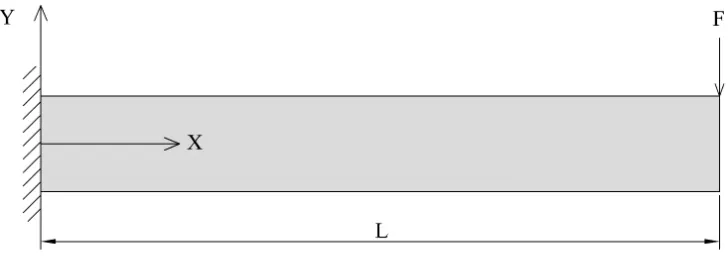
The presented QAGFVA is performed on a two-dimensional fixed–free cantilever beam supporting the concentrated load at the free end (Timoshenko and Goodier 1982; Afshar et al. 2012) which schematic figure is shown in Figure 12. Parameters h, b and l are the height, width and length of the cantilever beam, respectively. F is the applied concentrated load at the free end.

Fig. 12. Schematic illustration of the cantilever under concentrated load

According to analytical results, the horizontal and vertical displacement along X–axis are given as (Timoshenko and Goodier 1982):

(

) (

)

(

)

(

)

(

)

2 2

2

2 2

3 2 2

6 4

3 3 4 5

6 4

x

y

Fy h

u x l x y

EI

Fy h

u x l x l x y x

EI

υ

υ υ

  

= _ − + + _ − _

 

 

 

= − _ − + − + + _

 

(31)

in which, E, I are the Young’s modulus and the moment of inertia, respectively. The stress in x and y directions and the shear stress filed are calculated as follows:

(

)

2 3

2

, 0, ;

2 4 12

x y xy

F l x y F h _{y I} bh

I I

σ = − σ = σ = − _ − _ =

  (32)

Owing to the fact that the analytical solution is independent of the Poisson’s ratio, it is applicable to the cantilever beam under pure flexure (Timoshenko and Goodier 1982). Therefore, Poisson’s ratio is assumed to be zero in the QAGFVA. The geometrical and mechanical properties of the test case are presented in Table 3.

Geometrical Properties Mechanical Properties

Length l=12.0m _{Young ‘s Modulus} E=1000 Pa

Width b=1.0m _{Point Load} F=1N

Height h=2.0m _Density 2600 kg₃

m ρ=

Table 3. Geometrical and Mechanical Properties for a Cantilever

initial mesh is adapted during the adaptive analysis and finally an adaptive mesh, which contains the desired target relative error (10%), is obtained. The refined mesh is depicted in Figure 14.

Fig.13. Unstructured initial mesh for QAGFVA

Fig.14. The refined mesh for cantilever

By applying a 1N load, the maximum computed displacement, and the maximum bending stress are equal to 0.90 m, 17.7 Pa, respectively. The maximum displacement occurs at the free end. The computational results of the QAGFVA presents approximately 2% deviation from the analytical solution.

Comparison of the vertical displacement, uy, and stress in x direction, σx, (along the upper

surface of the beam) with the analytical results are presented in Figure 15. As shown in Figure 15, the computed results of the present modeling show good agreements with the analytical solutions.

Fig.15. Variation of the computed results along X axis

Method Number of _Nodes Number of _Elements CPU Time _(Second)

Adaptive Finite Volume 2000 3660 11.6

Adaptive Finite Element

Direct 1997 3649 108

Iterative

(GMRES) 2001 3667 9.15

Table 4. Comparison of CPU time for adaptive analysis using different numerical methods

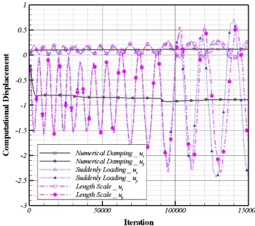
To have a good perspective on the convergence procedure, the computed displacements in x, y directions are presented in Figure 16. Additionally, the logarithm of root mean square of the computed displacement in x direction is shown in Figure 17.

Fig.16. Convergence of the computed displacements

Fig.17. Convergence of the logarithm of root mean square of the displacements in direction x

Fig.18. The error distribution of the cantilever beam

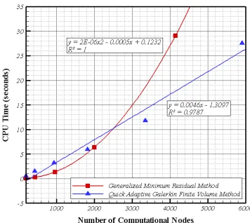
The CPU time of structural analysis using the QAGFVA and the GMRES methods is depicted in Figure 19. As it can be seen, the efficiency of the GMRES is significantly reduced when the number of computational nodes increases, but the QAGFVA maintains its efficiency. So the QAGFVA is the suitable method for large scale structures.

Fig.19. Computational time comparison between the iterative methods, the QAGFVA and GMRES Method

6. Conclusion

convenient implementation and fast numerical computation are the other merits of the introduced relation.

Following the adaptive mesh refinement strategies, which have been implemented in the context of the Finite Element Method, the h–refinement technique is adopted for the shape-function-free QAGFVA. A posteriori error estimator, which is based on the superconvergent patch recovery, is used to predict the regions of high error.

The numerical results show that the QAGFVA requires less CPU time in comparison to direct and indirect Finite Element Analyses. The presented results confirm that the QAGFVA not only is an accurate numerical solution, but also has a better performance, especially in meshes with large number of nodes.

References

Afshar M H, Amani J, Naisipour M (2012). A node enrichment adaptive refinement in discrete least squares meshless method for solution of elasticity problems. Engineering Analysis with Boundary Elements. 36: 385–393.

Alkhamis M T, Sabbagh–Yazdi S R, Esmaeili M, Wegian F M (2008). Utilizing NASIR Galerkin finite volume analyzer for 2D plane strain problems under static and vibrating concentrated loads. Jordan Journal of Civil Engineering. 2(4): 335–343.

Bank R E, Weiser A (1985). Some a posteriori error estimates for elliptic partial differential equations. Mathematics of Computation. 44(170): 283–301.

Bank R E, Smith R K (1993). A posteriori error estimates based on hierarchical bases. SIAM Journal on Numerical Analysis. 30(4): 921–935.

Boroomand B, Zienkiewicz O C (1999). Recovery procedures in error estimation and adaptivity, Part II: adaptivity in nonlinear problems of elasto–plasticity. Computer Methods in Applied Mechanics and Engineering. 176: 127–146.

Chang W, Kikuchi N (1994). An adaptive remeshing method in the simulation of resin transfer molding (RTM) process. Computer Methods in Applied Mechanics and Engineering. 112: 41–68.

Demirdžić I, Martinović D (1993). Finite volume method for thermo–elasto–plastic stress analysis. Computer Methods in Applied Mechanics and Engineering. 109: 331–349.

Ekhteraei–Toussi H, Rezaei–Farimani M (2007). Comparative analysis using the numerical methods of finite element, boundary element, element free Galerkin and finite volume in the field of solid mechanics. Proceedings, International Conference on Engineering and Mathematics, Spain.

Flaherty, J E (2005). Chapter 8: Adaptive Finite Element Techniques, available at: http://www.cs.rpi.edu/~flaherje/pdf/fea8.pdf

Gharehbaghi S A, Khoei A R (2008). Three–dimensional superconvergent patch recovery method and its application to data transferring in small–strain plasticity. Computational Mechanics. 41: 293–312.

Hay A, Visonneau M (2007). Adaptive finite–volume solution of complex turbulent flows. Computers & Fluids. 36: 1347–1363.

Ilinca C, Zhang X D, Trépanier J Y, Camarero R (2000). A comparison of three error estimation techniques for finite–volume solutions of compressible flows. Computer Methods in Applied Mechanics and Engineering. 189: 1277–1294.

Jasak H, Gosman A D (2000a). Automatic resolution control for the finite–volume method, part 1: a–posteriori error estimates. Numerical Heat Transfer B. 38: 237–256.

Jasak H, Weller H G (2000c). Application of the finite volume method and unstructured meshes to linear elasticity. International Journal for Numerical Methods in Engineering. 48: 267– 287.

Jasak H, Gosman A D (2003). Element residual error estimate for the finite volume method. Computers & Fluids. 32: 223–248.

Katragadda P, Grosse I R (1996). A posteriori error estimation and adaptive mesh refinement for combined thermal–stress finite element analysis. Computers & Structures. 59(6): 1149–1163. Kelley C T (1995). Iterative methods for linear and nonlinear equations. SIAM, Philadelphia. Khoei A R, Azadi H, Moslemi H (2008). Modeling of crack propagation via an automatic

adaptive mesh refinement based on modified superconvergent patch recovery technique. Engineering Fracture Mechanics. 75: 2921–2945.

Lee C Y, Oden J T (1994). A posteriori error estimation of h–p finite element approximations of frictional contact problems. Computer Methods in Applied Mechanics and Engineering. 113: 11–45.

Li X D, Wiberg N E (1994). A posteriori error estimate by element patch post–processing, adaptive analysis in energy and 𝐿𝐿2 norms. Computers & Structures. 53(4): 907–919.

Liu J, Mu L, Ye X (2011). An adaptive discontinuous finite volume method for elliptic problems. Journal of Computational and Applied Mathematics. 235: 5422–5431.

Lötstedt P, Ramage A, Sydow L V, Söderberg S (2004). Preconditioned implicit solution of linear hyperbolic equations with adaptivity. Journal of Computational and Applied Mathematics. 170: 269–289.

Meguid S A (1986). Finite element analysis of defence hole systems for the reduction of stress concentration in a uniaxially–loaded plate with two coaxial holes. Engineering Fracture Mechanic. 25(4): 403–413.

Meyer A, Rabold F, Scherzer M (2006). Efficient Finite element simulation of crack propagation using adaptive iterative solvers. Communications in Numerical Methods in Engineering. 22: 93–108.

Muzaferija S, Gosman D (1997). Finite-Volume CFD procedure and adaptive error control strategy for grids of arbitrary topology. Journal of Computational Physics. 138: 766–787. Palani G S, Iyer N R, Dattaguru B (2006). New a posteriori error estimator and adaptive mesh

refinement strategy for 2D crack problems. Engineering Fracture Mechanics. 73: 802–819. Phongthanapanich S, Dechaumphai P (2004). Adaptive Delaunay triangulation with object–

oriented programming for crack propagation analysis. Finite Elements in Analysis and Design. 40: 1753–1771.

Reddy J N, Gartling D K (2010). The finite element method in heat transfer and fluid dynamics. Third ed, CRC Press.

Sabbagh–Yazdi S R, Alimohammadi S (2009). Comparison of finite element and finite volume solvers results for plane–stress displacements in plate with oval hole. Proceedings, 4th International Conference on Continuum Mechanics, England.

Sabbagh–Yazdi S R, Amiri–SaadatAbadi T (2013). GFV solution on UTE mesh for transient modeling of concrete aging effects on thermal plane strains during construction of gravity dam. Applied Mathematical Modelling. 37: 82–101.

Sabbagh–Yazdi S R (2016). http://wp.kntu.ac.ir/syazdi/index.html, (accessed 18.01.10)

Sharif N H, Wiberg N E (2002). Adaptive ICT procedure for non–linear seepage flows with free surface in porous media. Communications in Numerical Methods in Engineering. 18: 161– 176.

Tabarraei A, Sukumar N (2005). Adaptive computations on conforming quadtree meshes. Finite Elements in Analysis and Design. 41: 686–702.

Thompson J F, Soni B K, Weatherill N P (1999). Handbook of grid generation. CRC Press, Florida.

Timoshenko S P, Goodier J N (1982). Theory of elasticity. McGraw–Hill.

Versteeg H K, Malalasekera W (2007). An introduction to computational fluid dynamics, the finite volume method. Bell & Bain Limited, Glasgow.

Yip S (2005). Handbook of materials modeling, volume I: methods and models. Springer. Zienkiewicz O C, Zhu J Z (1987). A simple error estimator and adaptive procedure for practical

engineering analysis. International Journal for Numerical Methods in Engineering. 24: 333– 357.

Zienkiewicz O C, Boroomand B, Zhu J Z (1999). Recovery procedures in error estimation and adaptivity, Part I: adaptivity in linear problems. Computer Methods in Applied Mechanics and Engineering. 176: 111–125.