Spline Interpolation Techniques
Erdogan KAYA*
Abstract
This article belongs to an area of computer technologies and engineering, and discusses four different spline interpolation meth-ods (linear, quadratic, cubic and cubic Hermite) for chemical engineering application, applied on spray dryer case. In the article GUI (graphical user interface) is coded in Matlab. It is designed to test four interpolation methods and compares them. Within Mat-lab, GUI tools enable you to perform tasks such as creating and customizing plots, curves and surfaces, and analyzing and filtering signals. In the article, interpolation techniques are discussed by using the data sets from any experimental results. Finally, A Spline GUI is developed for the end-users to interpolate their own experimental data sets. Users need to enter their experimental data to the screen. After that by clicking push buttons, they can plot the spline method desired. If the user clicks on the check button, answers can be plotted in an external figure window as well. The figure can be saved or copied to Clipboard.
Keywords: interpolation, splines, linear spline, quadratic spline, cubic spline, cubic hermite spline, GUI, MATLAB
Introduction
In practical fields such as medicine, physics, engineering and computer graphics the amount of data obtained through ex-perimental or statistical surveys is usually very large. The use of an interpolation scheme for the construction of spline curves from the given data consisting of a relatively large number of points will yield a huge number of curve segments. On the oth-er hand, in most applications the points are subject to measure-ment errors. We can hope that with the curve approximation, these errors will be smoothed out and the resulting curve will look smooth enough.
Before the inventing of calculators mathematical tables were a necessity for everybody applying mathematics. Inter-polation was first used to calculate additional values based on tabulated values of special functions.
The approximation theory is one of the main topics of numerical analysis. It is a foundation for numeral algorithms in the different fields of applied mathematics. Polynomial in -terpolation is especially important, since it offers an approxi-mating function in a closed form, which is widely used in implementations. Polynomials are the most easily handled in practice, since they can be represented by restricted informa-tion, evaluated in limited number of basic operations and easily integrated or differentiated.
In recent years, splines have attracted attention of both researchers and users who need various approximation tools. To sum up, linear splines are a set of joint line segments, a continuous function with discontinuous first derivative at the knots. Quadratic splines have a continuous first derivative, cu -bic splines continuous first and second derivatives, and so on. Linear splines are evidently too rough of an approximation to a physical spline, a cubic spline is adequate, quartic and higher order splines are possible but require more computation. (Th-erneau M, 2000)
Interpolation
Interpolation is an estimation of a value within two known values. It is an estimation of an unknown quantity between two known quantities or drawing conclusions about missing infor-mation from the available one. Interpolation is useful where the data surrounding missing data is available and where longer-term cycles are known. Interpolation is a method of building a function that crosses through a discrete set of known data points.
There are many different interpolation methods (four of them are discussed below). While choosing an appropriate al-gorithm and interpolation method some of the concerns should be foreseen, for example how accurate is the method, how smooth is the interpolate or how many data points are needed and etc.
Linear Interpolation
Linear interpolation has been used for filling the gaps in tables, often with astronomical data. It is believed that it was used by Babylonian astronomers, by mathematicians in Seleu-cid Mesopotamia, and by the Greek astronomer and mathema-tician, Hipparchus. A description of linear interpolation can also be found in the Almagest by Ptolemy.
The linear splines are much simpler than cubic splines. The result of linear interpolation is a set of straight lines connect-ing the data points. For two spatial dimensions, the extension of linear interpolation is called bilinear interpolation. In three dimensions it is called tri-linear interpolation. (Carpenter K. H. 1999)
This method is often used in chemical engineering since the resulting spline never overshoots. Even so, when a smooth interpolate is desired, a higher order spline is needed.
The fundamental operation of linear interpolation between two values is widely used in computer graphics, it is sometimes called as a lerp. Lerp operations are constructed on the hard-ware of all modern computer graphics processors. They are of-ten used as constructing blocks for more complex operations, * Master student, Faculty of Computer Technologies and Engineering, International Black Sea University, Tbilisi, Georgia.
for example, a bilinear interpolation can be accomplished in three lerps. Because this operation is not expensive, it’s also a good way to implement accurate lookup tables with quick lookup for smooth functions without having too many table entries.
Linear spline models are criticized because of the abrupt change in trend going from one segment to the next, which does not represent what would naturally occur. The true change in trend should be smooth. In mathematical terms this means that the fitting function should have a continuous derivative at each value of the independent variable. This is not possible for linear splines, but it is possible for quadratic splines that are joined segments of parabolas. (Z. Huang and J. Stone, 1999)
Quadratic Spline
A quadratic spline interpolation method produces a better fit to a continuous function than a linear spline does. A quad -ratic spline is a continuously differentiable piecewise quad-ratic function, where quadratic includes all linear combinations of the basic monomials.
Quadratic splines are not used in applications as much as natural cubic splines. However, the derivations of interpolating quadratic and cubic splines are similar enough, so that an un-derstanding of the simpler second-degree spline theory allows us to grasp easily the more complicated third-degree spline theory. (Cheney W. and Kincaid D.)
Cubic Spline
Cubic splines play an important role in fields where smooth interpolation is essential, in modeling, for example, animation and image scaling. In computer graphics interpolating cubic splines are often used to define smooth motion of objects and cameras passing through user-specified positions in a key frame animation system. In image processing splines prove useful in implementing high-quality image magnification.
Cubic Hermite Spline Interpolation
There are many kinds of piecewise polynomial interpola-tion. We can try to modify a set of cubic splines with a set of other polynomials such as the cubic Hermite polynomials. These cubic Hermite polynomials allow us to provide not only continuity of the first order derivatives of the curve but also to match the set of chosen slopes. This interpolation is appropriate when both the function and the derivative values are available.
In the mathematical field of numerical analysis a cubic Hermite spline, named after Charles Hermite, is a third-degree spline in Hermite form. The Hermite form has two control points and two control tangents for each polynomial. They are simple to calculate but at the same time too powerful. (Gras-selli, M., Pelinovsky, D., 2008)
Theoretical Background on Cubic Hermite Theory
Cubic Hermite interpolation is the most common piece-wise polynomial method. It is considered as piecepiece-wise since a unique polynomial is fitted between all data points. Also, each of these polynomials ate linked to adjacent polynomials by us-ing a set of constrains. This collection of polynomials that form the curve is jointly considered as the spline.
Depending on the type of mathematical constrains placed upon the Hermite splines, different member in the Hermite fam-ily can be made. For example, the traditional and constrained Hermite splines are two different groups of the same family. Many more groups in this family can be determined by appro-priately modifying constrains. The group of traditional Hermite splines can be divided into subgroups, for example natural, par-abolic run-out, Hermite run-out and clamped Hermite splines. The natural Hermite spline is the most popular and widely used version of Hermite spline family. (Greef, P., 2003)
The essential theory underlying any spline is to fit piece -wise function of the following form:
On the interval in the case of cubic Hermite in-terpolation, is a third order or cubic polynomial defined as follows:
The first and the second order derivatives of these poly -nomials are fundamentally important in this process and are given by:
and
for i=1,2,….n-1
Based on equations above four mathematical constrains that characterize the constrained Hermite Splines can be de-fined as follows:
• The piecewise function will interpolate all data points on the interval and therefore:
for i=1,2,…,n.
• Since the curve must be continuous on the in-terval , each piecewise polynomial should join at shared node points:
for i=2,…,n-1.
Constrained curve has noticeably less smoothness tan the natural curve, but succeeds in its goal of not overshooting in any region between node points. Constrained curve interpo-lates the region linearly instead of cubically like the natural curve. (Greef, P., 2003)
The degree to which both Hermite spline interpolation methods compare to ordinary linear interpolation can be quali-fied by taking the absolute difference between the two yields calculating using the Hermite Spline and linear interpolation methods. If the linear interpolated curve is taken to be favored discontinuous yield curve, the constrained Hermite spline de-viates considerably less from it compared to natural Hermite spline.
If A specified first order derivative, or slope, at every point,
A relatively simple equation that works well and satisfies these requirements is:
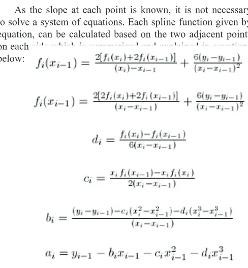
As the slope at each point is known, it is not necessary to solve a system of equations. Each spline function given by equation, can be calculated based on the two adjacent points on each side which is summarized and explained in equations below:
Or it can be written in a so-called Bernstein-Bezier form: (Kruger, CJC)
Shape preservation is an important factor in graphical dis-play of the data. In last years, huge amount of articles have been published by scientists in the field. The issues of shape preservation have been argued. Convexity, monotonicity and non-negativity preserve the shape of the data and make it visu-ally pleasing.
The monotonicity issue has been investigated by number
of mathematicians. M. Sarfraz and M. Hussain have found an interpolation by rational cubic functions with four degree of freedom and they provided very visually pleasant curves. This work is particularly interested with the convexity, monotonic-ity and positivmonotonic-ity of the data using the rational cubic function with four shape parameters, that provide extra independence to the user to modify the curves. Two of the parameters control shape of the curves, while the other two refine the curve as desired by the user. (Dougherty R. L. 1989)
In Fritsch and Carlson’s “Monotone Piecewise Cubic In -terpolation” necessary and sufficient conditions are derived for a cubic spline to be monotone on an interval. These conditions are used to develop an algorithm which constructs a visually pleasing monotone piecewise cubic interpolant to monotone data. The algorithm which is described in the article is simple, and the interpolant is affected only locally by changes in the data.
According to Akima’s “A New Method of Interpolation and Smooth Curve Fitting Based on Local Procedures” a new mathematical method is developed for interpolation for a given set of data points. This method is devised in such a way that the resultant curve will pass through the given points and will appear smooth and natural. In the article the slope of the curve is determined at each given point locally, and each polynomial represents a portion of the curve between a pair of given points by the coordinates of and the slopes at the points (Akima H. 1970)
Carl De Boor suggests a cubic spline interpolate that pre-serves the convexity of data by inserting additional breakpoint between each pair of data points. However the approach does not guarantee monotonicity (De Boor C. 1978)
Experimental Results
Results of experiments with different flow rates vs pump power are given below where we use Linear, Quadratic, Cubic and Cubic Hermite Spline interpolation techniques to fit the data.
Spray Dryer Data is given in the Table below. The table shows the results of grape seed extract for different pump pow-er and flow rate values.
For the values in the table containing experimental data, dif-ferent spline interpolation methods are demonstrated. For specific type of data, I observed and discussed advantages and disadvantages of different methods. A friendly user interface GUI was developed in order to simplify the choice of the ap-propriate method for the user’s data
Linear spline interpolation method was used to fit the data in MATLAB GUI. As shown in Figure 1, linear spline has hardly any smoothness. It preserves the local monotonicity of the data and never overshoots. That is why it is widely used and very famous in chemical engineering applications.
Figure 1: Linear Spline
For the given data, we used quadratic spline interpolation method in MATLAB GUI. As shown in the Figure 2, quad-ratic spline oscillates and overshoots too much. Because of it quadratic splines are rarely used for interpolation for practical purposes. Ideally quadratic splines are only used to understand cubic splines.
Figure 2: Quadratic Spline
Next, we used natural cubic spline interpolation method in MATLAB GUI. As shown in the Figure 3, cubic spline has two continuous derivatives, which provides visually pleasing rep-resentation of the function. But at the same time, natural cubic spline can’t guarantee to preserve shape and sometimes it oscil -lates and overshoots. In this case, it’s better to use linear spline. Figure 3: Cubic Spline
Finally, cubic Hermite spline interpolation method was used to fit the data in MATLAB GUI. As shown on the Fig-ure 4, cubic Hermite spline has one continuous derivative, it guarantees to preserve shape, never oscillates and overshoots. If function and derivative values are given in advance, Her-mite spline is faster than cubic spline, otherwise it is twice as expensive.
Figure 4: Cubic Hermite Spline
To illustrate the differences three interpolants, linear, cu-bic and cucu-bic Hermite, are shown in the Figure 5, (quadratic interpolation method is not included because of too much os-cillation).
Figure 5: Combination of Linear, Cubic and Cubic Hermite
As Figure 5 shows, cubic Hermite interpolant has more pleasing visual appearance than linear and cubic; also it allows flexibility to preserve monotonicity.
Spline Method Evaluator
A Graphical User Interface (GUI) allows users to perform tasks interactively through controls such as buttons and sliders. Within Matlab environment, GUI tools enable us to perform tasks such as creating and customizing plots, fitting curves and surfaces, and analyzing and filtering signals. One can create custom GUIs for others purposes as well.
GUIDE(GUI development environment) provides tools for designing and programming GUIs. Using the GUIDE Layout Editor, one can graphically design his GUI. GUIDE then au-tomatically generates MATLAB code, that defines all compo -nent properties, and establishes a framework for GUI callbacks (routines that are executed, when a user interacts with a GUI component). In Figure 6, an example of GUI is shown.
GUI components can include menus, toolbars, push but-tons, radio butbut-tons, list boxes, and sliders. GUIs created
ing MATLAB tools can also perform any type of computation, read and write data files, communicate with other GUIs, and display data as tables or as plots.
Our GUI contains, four axes components, a pop up menu listing colors of lines, static texts, and several buttons that pro-vide control over different kinds of plots, grids, etc. A picture of the GUI, Spline Method Evaluator with data, is shown in Figure 7.
We coded the GUI by using MATLAB R2010a. IBSU Logo is embedded in GUI Layout with the help of axes. GUI is designed to test four different spline methods and compare them. Here are some of the tasks performed by a user and GUI.
• Users need to enter their experimental data to the screen;
Figure 7: Graphical User Interface with Data
• After that by clicking push buttons, they can plot the spline method desired. If the user clicks on the check button, answers can be plotted in an external figure window as well. In Figure 8, an external graph is plotted for Cubic Spline;
• The figure can be saved or copied neatly to clipboard; • There is an edit menu for figures. If you open a plot -ted line, the figure can be manipula-ted in various ways such as changing title, label, legend, line style and copying to clip-board for pasting to Microsoft Word, and Excel, etc. This is not true for some other situations. Suppose you run your GUI application in the Matlab Command Console. If you embed a plot inside a GUI layout, lines in the figure cannot be edited unlike in a plot in a separate figure window. Suppose you run a compiled stand alone application. It is known to developers that there is only a File menu. It can only be used to save or print a figure. It cannot be used to manipulate the figure in any way except for zooming or rotating. It cannot be even copied
to clipboard for pasting. Add figure menu was created by Dr. Tingyue Gu and used in my application. It adds extra menu items so that a figure can be manipulated directly once a figure is created by a stand alone application without using MATLAB command console. By right clicking on the mouse, edit menu can be activated as it is shown in Figure 9;
• There is a Clear Button to refresh the data;
• There is a Quit Button which closes the application; • By using Grid On and Off Buttons, users can turn on and off grids for the graphs.
Figure 9: Interactivity in Graphical User Interface
Conclusion
Chemical Engineers deal with a lot of data that are crucial for modeling, process analysis, and process design. Data are often obtained or given for discrete values along a continuum, from which we often require a trend analysis or estimates at in-termediate points. If we are developing a mathematical model for a certain process or physical phenomenon, we may also need to obtain some model parameters fitted to experimental data. The procedure that we need for these purposes is called curve fitting.
Based on our observations for the data we have used, in-formation from Flow Rate vs Pump Power Table, we conclude: • Linear Spline is a good way of representing spray dryer results. Because it never overshoots the data and preserves mo-notonicity. The drawback of Linear Spline is, it is not smooth, Figure 6: Graphical User Interface
and it does not represent the real behavior of the function. • Quadratic Splines oscillates and overshoots the data ex -tremely, it does not have any scientific value for our data.
• Cubic Splines are visually pleasing. Even though they may oscillate for some data, they produce reasonable fit to the data we used.
• For our spray dryer results, Cubic Hermite is showing the best behavior. It does not overshoot, it preserves the shape, it is smooth and monotonic.
As a result, for this specific Flow Rate Data, Cubic Her -mite is chosen as the best curve fitting approximation method.
References:
[1] Gibb, D.,2012, A Course in Interpolation and Numerical Integration for the Mathematical Laboratory, HardPress, New York
[2] Grasselli, M., Pelinovsky D.,2008, Numerical Mathemat-ics, Jones and Bartlett Publishers, USA
[3] Therneau, T. M., Grambsch P. M.,2000 Modeling survival data (Extending the cox model), Springer, New York, USA [4] Wolberg, G, Alfy I.,2001 An energy-minimization frame-work for monotonic cubic spline interpolation, Journal of Computational and Applied Mathematics, Department of Computer Science, City College of New York, New York, NY 10031, USA
[5] Greef, P.2003, Applying Constrained Cubic Splines to Yield Curves, Think Notes, Riscura
[6] Terry M. Therneau, Patricia M. Grambsch, Modeling sur-vival data (Extending the cox model), Springer, 2000, 100-120 [7] Kenneth H. Carpenter, An introduction to interpolation and splines, EECE KSU, November 22, 1999 revised November 20, 2001, April 24, 2002, April 14, 2004, 1-8
[8] Jianhua Z. Huang and Charles J. Stone, Extended Linear Modeling with Splines, 1999, 1-20
Ward Cheney, David Kincaid, Numerical Mathematics and Computing, seventh edition, 250-260
[9] Randall L. Dougherty, Alan Edelman, James M. Hyman, Nonnegativity, Monotonicity, or Convexity-Preserving Cubic and Quintic Hermite Interpolation,J-Stor April, 1989
[10] H.Akima, A New Method of Interpolation and Smooth Curve Fitting Based on Local Procedures, Journal of the ACM (JACM), Volume 17, Issue 4, Oct. 1970, Pages 589-602