A time series classifier

Masters Theses Student Theses and Dissertations Spring 2008

A time series classifier

A time series classifier

Follow this and additional works at: https://scholarsmine.mst.edu/masters_theses

Part of the Computer Sciences Commons Department:

Department:

Recommended Citation Recommended Citation

Gore, Christopher Mark, "A time series classifier" (2008). Masters Theses. 4609.

https://scholarsmine.mst.edu/masters_theses/4609

This thesis is brought to you by Scholars' Mine, a service of the Missouri S&T Library and Learning Resources. This work is protected by U. S. Copyright Law. Unauthorized use including reproduction for redistribution requires the permission of the copyright holder. For more information, please contact [email protected].

by

CHRISTOPHER MARK GORE

A THESIS

Presented to the Faculty of the Graduate School of

MISSOURI UNIVERSITY OF SCIENCE AND TECHNOLOGY in Partial Fulfillment of the Requirements for the Degree

MASTER OF SCIENCE IN COMPUTER SCIENCE

2008 Approved by

Daniel R. Tauritz, Advisor Ralph W. Wilkerson

ABSTRACT

A time series is a sequence of data measured at successive time intervals. Time series analysis refers to all of the methods employed to understand such data, either with the purpose of explaining the underlying system producing the data or to try to predict future data points in the time series. Time series analysis is applicable to many problems since there are so many areas that require a more thorough understanding of a time series or the prediction of future values of the time series. The most typical historical examples of time series would be the weather and the financial markets but there are many more real-world time series problems.

An evolutionary algorithm is a non-deterministic method of searching a solution space, and modelled after biological evolutionary processes. A learning classifier system (LCS) is a form of evolutionary algorithm that operates on a population of mapping rules. We introduce the time series classifier TSC, a new type of LCS that allows for the modeling and prediction of time series data, derived from Wilson’s XCSR, an LCS designed for use with real-valued inputs. Our method works by modifying the makeup of the rules in the LCS so that they are suitable for use on a time series. All of the operations (mutation, crossover, etc.) applied to the rules also were changed from their traditional forms.

We tested TSC on real-world historical stock data. The system would always return a profit, but not as much as the stock market itself is capable of returning by the utilization of an indexing fund. The stock market is a notoriously difficult system to model effectively and therefore any positive results at all are notable, and never losing money in the long-term is impressive in itself, often a difficult task for unskilled human traders.

Although this initial system appears incapable of producing monetary returns better than that of the stock market itself and may not be the eventual solution, it does perform well enough to demonstrate that the system is capable of learning in a very complex envi-ronment. The inherent complexity of the market makes the system unusable for automated trading, but this approach should prove to be useful in other less challenging real-world time series problems.

ACKNOWLEDGMENTS

I would like to thank for all of their support and help my parents Charles and Carolyn Gore, my wife Monica, and my advisor Daniel Tauritz.

TABLE OF CONTENTS

Page

ABSTRACT . . . iii

ACKNOWLEDGMENTS . . . iv

LIST OF ILLUSTRATIONS. . . vii

LIST OF TABLES. . . viii

LIST OF ALGORITHMS. . . ix SECTION 1. INTRODUCTION . . . 1 1.1. MOTIVATION . . . 1 1.2. BACKGROUND . . . 2 1.3. REINFORCEMENT LEARNING. . . 2

1.3.1. Exploration versus Exploitation . . . 3

1.3.2. The Whole Problem . . . 3

1.4. EVOLUTIONARY ALGORITHMS . . . 3

1.4.1. Learning Classifier Systems . . . 4

1.4.2. ZCS . . . 5

1.4.3. XCS . . . 8

1.4.4. XCSR . . . 10

2. TIME SERIES PREDICTION. . . 12

2.1. ARIMA AND OTHER STATISTICAL METHODS . . . 12

2.2. ARTIFICIAL NEURAL NETWORKS . . . 13

2.3. NON-LCS EVOLUTIONARY APPROACHES . . . 14

2.4. LCS-BASED APPROACHES . . . 14

2.4.1. XCS . . . 14

2.4.2. XCSF . . . 14

3. APPROACH AND DESIGN OF THE TIME SERIES CLASSIFIER . . . 16

3.1. FUNDAMENTAL OPERATIONS . . . 16

3.1.1. The Sort On Algorithm . . . 16

3.1.2. The Sort Order Algorithm . . . 17

3.1.3. Rasterized Linear Paths Through Arrays . . . 17

3.1.3.2. A purely vertical path. . . 18

3.1.3.3. A traditional diagonal path. . . 18

3.1.3.4. Non-equal diagonal paths. . . 19

3.1.3.5. The Raster Line Algorithm. . . 19

3.1.4. List Slices . . . 20 3.2. DATA REPRESENTATION . . . 21 3.3. RULE REPRESENTATION . . . 22 3.4. MUTATION . . . 22 3.5. CROSSOVER. . . 23 3.6. LEARNING PARAMETERS . . . 23 3.6.1. From XCS . . . 23 3.6.1.1. General Parameters . . . 23 3.6.1.2. Recalculating Fitness . . . 24 3.6.1.3. Multi-Step Specific . . . 24 3.6.1.4. GA Specific . . . 24

3.6.1.5. Rule Set Specific. . . 25

3.6.2. From XCSR . . . 26

3.6.3. New in TSC . . . 27

3.7. TRIVIALLY MODIFIED ALGORITHMS . . . 27

3.8. THE MATCH? PREDICATE . . . 30

3.9. THE GENERATE COVERING CLASSIFIER ALGORITHM . . . 31

3.10.THE MORE GENERAL? PREDICATE . . . 31

4. EXPERIMENTAL RESULTS . . . 33

4.1. THE NATURE OF A REALISTIC TIME SERIES. . . 33

4.2. THE SIMPLISTIC INCREASING/DECREASING TESTS . . . 33

4.3. THE STOCK MARKET . . . 34

4.3.1. Reward Methods . . . 36

4.3.2. GA Thresholds. . . 40

4.3.3. Crossover Probabilities . . . 41

4.3.4. Mutation Probabilities . . . 43

4.3.5. Exploration Probabilities . . . 46

5. CONCLUSIONS AND FINAL RESULTS . . . 48

6. FUTURE WORK. . . 50

BIBLIOGRAPHY . . . 53

LIST OF ILLUSTRATIONS

Figure Page

1.1 ZCS’s basic structure . . . 6

1.2 XCS’s basic structure . . . 9

1.3 XCSR’s interval rules. . . 11

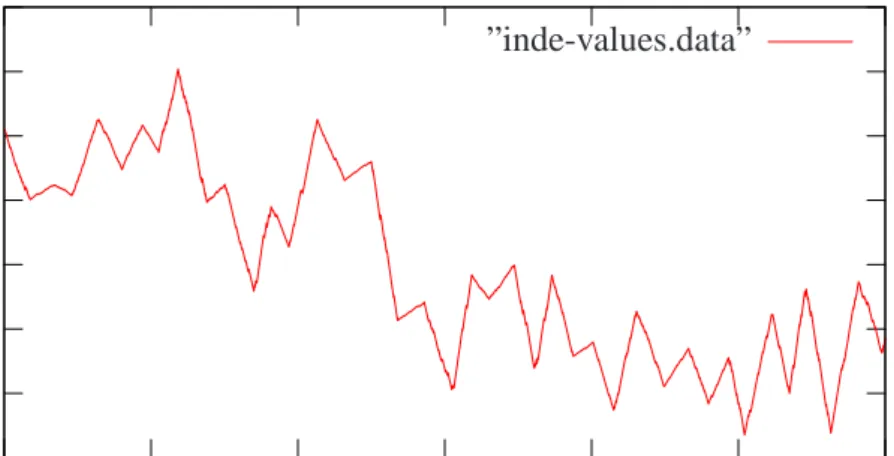
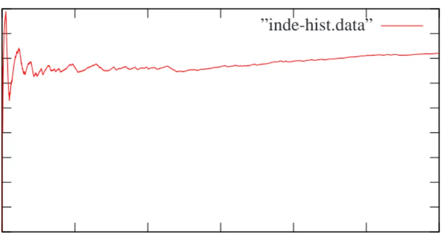
4.1 Increasing/decreasing method 4 sample plot. . . 34

LIST OF TABLES

Table Page

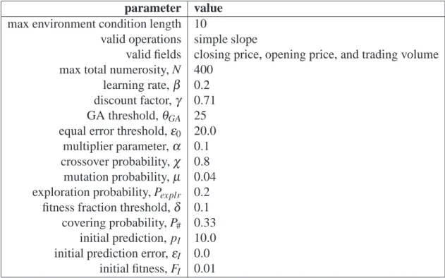
4.1 Initial parameters for the TSC. . . 36

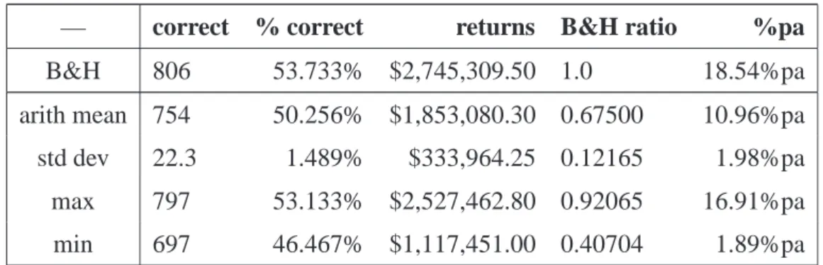
4.2 TSC results for reward method a1. . . 37

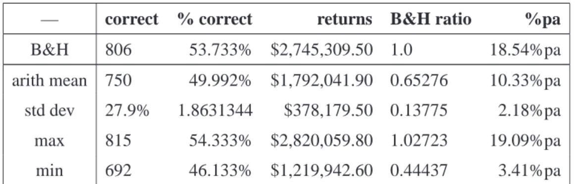
4.3 TSC results for reward method a2. . . 37

4.4 TSC results for reward method b. . . 38

4.5 TSC results for reward method c. . . 38

4.6 TSC results for reward method dopt. . . 39

4.7 TSC results for reward method dpess. . . 40

4.8 TSC results for a GA threshold of 35. . . 40

4.9 TSC results for a GA threshold of 45. . . 41

4.10 TSC results for a GA threshold of 50. . . 41

4.11 TSC results forχ=0.3. . . 42 4.12 TSC results forχ=0.5. . . 42 4.13 TSC results forχ=0.7. . . 43 4.14 TSC results forχ=0.9. . . 43 4.15 TSC results forµ =0.06. . . 44 4.16 TSC results forµ =0.08. . . 44 4.17 TSC results forµ =0.10. . . 45 4.18 TSC results forµ =0.15. . . 45 4.19 TSC results forµ =0.20. . . 45

4.20 TSC results for P_explr=0.1.. . . 46

4.21 TSC results for Pexplr=0.15. . . 46

4.22 TSC results for P_explr=0.3.. . . 47

4.23 TSC results for Pexplr=0.4.. . . 47

LIST OF ALGORITHMS

Algorithm Page

1.1 The evolutionary process. . . 4

3.1 Sort on. . . 17

3.2 Sort order. . . 17

3.3 Raster line. . . 20

3.4 List slice. . . 21

This thesis considers applying learning classifier systems (LCS’s) to the prediction of time series data. A time series as used here is a sequence of data successively measured through time. Time series analysis encompasses many methods that attempt to understand such time series, aimed at either understanding the underlying theory present in the data points or to make real-world predictions. Time series prediction is the use of a model to predict future events based on known past events: to predict future data points before they are measured. One standard example is the opening price of a share of stock based on its past performance.

1.1. MOTIVATION

No LCS to date has been designed for time series data but instead they were generally limited to Markov systems lacking any memory, which we viewed as a major limitation of LCS’s. LCS’s are designed specifically with the concept of evolving an effective rule set for a specified problem, which is specifically the sort of capability that would be desirable for time series analysis and prediction: generating useful rule sets.

An LCS is an evolutionary algorithm that operates on a population comprised of rules referred to as the rule set: this rule set is used to attempt to classify a situation. The first LCS was created by Holland [1] shortly after he created genetic algorithms (GA’s) [2], one of the classical types of evolutionary algorithms. Holland’s first LCS originally used a GA as the evolutionary device. Our system as described here also uses a GA for evolution, although it has been modified from the original form.

Holland’s original LCS was quite complicated and failed to produce quality results for most real-world problems. Because of this, the study of LCS’s was somewhat inactive until Wilson introduced ZCS [3], a re-imagining of Holland’s original LCS distilled to its most basic elements. Wilson’s ZCS was capable of producing acceptable results on certain problems and was simple enough to easily understand, reinvigorating LCS research.

A few years after introducing ZCS, Wilson modified it introducing XCS [4], which is currently one of the best performing and most popular LCS types. Wilson’s XCS was based on ZCS but with several important modifications mostly aimed at improving the accuracy of the rules produced and also for a more full coverage of the problem space by the rules. A significant portion of the LCS’s being worked on today are modifications or enhancements of Wilson’s XCS.

One such enhancement of XCS is known as XCSR [5], which was also developed by Wilson. XCSR improves upon XCS by allowing it to operate with real-valued ranges for input instead of on the traditional ternary alphabet so common to LCS’s, consisting of true, false, and a covering symbol (usually represented as # or∗).

1.2. BACKGROUND

The system presented here is derived from Wilson’s XCSR, which is an extension of Wilson’s XCS, which in turn was derived from Wilson’s ZCS. ZCS, XCS, XCSR, and this system are all learning classifier systems (LCS’s), a crossover of the fields of evolutionary computation (EC) and reinforcement learning (RL), both of which are quite large fields on their own. We will describe in this section the previous works this system was built upon.

1.3. REINFORCEMENT LEARNING

Reinforcement learning [6] is the process of learning how to map situations to actions to maximize a numerical reward. The learning system is not told which actions to take, as in most forms of machine learning, but instead must discover which actions yield the most reward by exploration. In the most interesting and challenging cases, actions may affect not only the immediate reward but also the next situation and, through that, all subsequent rewards. The two primary distinguishing characteristics of reinforcement learning are:

1. trial-and-error search and 2. delayed reward.

Reinforcement learning is defined not by characterizing learning methods, but by charac-terizing a learning problem. We consider any method that is well suited to solving that problem to be a reinforcement learning method. The idea is to capture the most important

aspects of the problem facing the learning agent interacting with its environment to achieve its goal. Such an agent must be able to:

1. perceive the state of the environment, 2. act on the environment, and

3. have a goal or goals relating to the state of the environment. Tersely put: sensation, action, and goal.

1.3.1. Exploration versus Exploitation. A primary challenge is the trade-off between exploration and exploitation. A reinforcement learning agent will prefer actions that it has tried in the past and found to be effective in producing reward in order to reliably obtain more reward. But to discover such actions, it has to try actions that it has not selected before. The agent has to exploit existing knowledge to obtain reward, but it also must explore to make better action selections in the future. Neither exploration nor exploitation can be pursued exclusively without failure. The agent must try a variety of actions and progressively favor those that appear to be best. On a stochastic task, each action must be tried many times to gain a reliable estimate of its expected reward.

1.3.2. The Whole Problem. Reinforcement learning explicitly considers the whole problem of a goal-directed agent interacting with an uncertain environment, start-ing with a complete, interactive, goal-seekstart-ing agent, instead of considerstart-ing subproblems without addressing how they might fit into a larger picture. All reinforcement learning agents have explicit goals, can sense aspects of their environments, and can choose actions to influence their environments. From the beginning, the agent operates with significant uncertainty about its environment. For learning research to make progress, important sub-problems have to be isolated and studied, but they should be subsub-problems that play clear roles in complete, interactive, goal-seeking agents, even if all the details of the complete agent cannot yet be filled in.

1.4. EVOLUTIONARY ALGORITHMS

In artificial intelligence (AI), evolutionary algorithms (EA’s) are a style of generic population-based meta-heuristic optimization algorithms whose processes are inspired by those of natural biological evolution. The primary mechanisms employed in EA’s to evolve a population of possible solutions towards an optimal one are:

1. parent selection based on fitness, 2. recombination,

3. mutation, and

4. and survivor selection based on fitness.

Evolution serves as a powerful metaphor and demonstrates great creativity in both the nat-ural world and in the world of computer science.

In normal biological evolution the environment that the population exists in exerts various pressures on the individuals in the population that determines the likelihood that any particular individual will manage to survive long enough to reproduce, and it is through this process that the fitness of an individual in the population must be determined: relative to its environment. In an EA, the environment relates to the problem we wish to solve, the individuals in the population encode potential solutions to that problem, and their fitness is their quality as a solution to the problem. By mimicking the methods of natural evolution in this manner we can often arrive at good solutions. The basic evolutionary process is outlined in Algorithm 1.1.

1. Initialize the population, either with randomly-generated or seeded candidate solutions or both.

2. Evaluate the fitness of each member of the population.

3. repeat

4. Select members of the population to act as parents. This is typically related to the relative fitness of the parents in some way.

5. Recombine the genetic material of the parents, producing offspring to be added to the population.

6. Mutate some or all of the newly-created offspring.

7. Evaluate the fitness of the offspring.

8. Select survivors from the current population or a subset thereof, often only the newly-created offspring, to survive to the next generation.

9. until some specified termination condition is satisfied.

1.4.1. Learning Classifier Systems. A learning classifier system is a type of EA in which a description of a current situation is used in an attempt to map that description to some classification or action. This is achieved through simulated evolutionary processes, where the population being evolved consists of various rules; our entire population forms a rule set, and we apply concepts from Darwinism to our individual rules. This is known in learning classifiers as the Michigan approach [7]. The other primary method employed, where each individual is an entire solution, and therefore a whole rule set, is known as the Pittsburgh approach. We use a modification of XCSR here, which uses the Michigan approach, and therefore so do we.

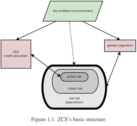
1.4.2. ZCS. ZCS is a zeroth level classifier system originally proposed in [3]. ZCS preserves most of the functionality of traditional LCS’s, but it is a very simplified version, which aids in the understanding of the classifier and its actions. This was a very useful contribution, because many of the problems with LCS’s before then were their overly complex and detailed nature. A good short summary of ZCS can be found in [7], and this summary is based primarily on that. The basic structure of ZCS is graphically illustrated in Figure 1.1.

In ZCS there is no message list, a much-welcomed simplification of the traditional LCS. This comes with a cost: there is no explicit method for transmitting information between cycles without the message list. This makes the interface entirely dependent on the interface of the system with its environment, and thus assumes a Markov process. This is most definitely an invalid assumption for real-world traded markets and for other time-series data.

Each rule r is of the form r= (c,a,s)where:

• c is the condition matched by the rule r and is comprised of elements from some alphabet, typically{0,1,#}, where # is the matching symbol, matching both 0 and 1; • a is the action that the rule r recommends;

• and s is the real-valued strength measurement of the rule r, s∈R_{, which determines}

how much of a vote rule r has in selecting the action to pursue.

In each time cycle t the match set Mt is found, a subset of the population, Mt ⊆P, with P being the entire population of rules, the rule set. The members at time cycle t of

Figure 1.1. ZCS’s basic structure

the match set Mt can be divided into disjoint subsets based on the action they recommend. With a finite set of possible actions

A ={_a0,_a1, . . .,_a|A|} ₍₁₎

andA′⊆A _where

A′_={a′

0,a′1, . . . ,a′|A′|} (2)

comprises all of the actions represented in the match set Mt. For any specific action a′i represented in the match set Mt we can form the set of all members of the match set that recommend action a′_i, represented as M_t,a′

i⊆Mt with

M_t,a′

i =

r : r∈Mt∧ar=a′i . (3)

The fitness of an action a′_i∈A′_{is then}

fitness(a′_i) =

∑

∀r∈M_t,a′

i

the sum of the fitness of all of the rules r that recommend that particular action present in M_t,a′

i. The action to take is selected in a fitness-proportionate method, choosing the action a′ with the greatest fitness. If Mt = /0 then covering must take place; a random rule that matches the current situation is created by initially setting c to exactly the current situation and then replacing a few elements of c at random with the # symbol, and that suggests a randomly-selected action.

The credit assignment scheme used by ZCS is somewhat involved, and is referred to as an implicit bucket brigade. It attempts to reward sequences which lead to reward from the environment and which are short. First, the rules in the population P but excluded from the match set Mt are originally unchanged:

s′_r=sr∀r∈/Mt. (5)

Next, the rules in the match set Mt but excluded from the action set At (those advocating weaker actions than the one chosen) have their strengths reduced by a factorτ ∈[0,1):

s′_r=τsr∀r∈Mt\At. (6)

Then the strength of the rules in the current action set At have a fractionβ ∈[0,1)of their strengths transferred to the members of the previous action set At−1, reduced by a factor

γ ∈[0,1):

s′_r= (1−β)sr∀r∈At, (7)

s′′_r =s′_r+γ∑∀r∈Atβsr

|At−1| ∀

r∈At−1. (8)

Finally, any feedback Pt from the environment is reduced byβ and distributed to the rules in the current action set At:

s′′′_r =s′′_r+βPt |At|

∀r∈At. (9)

A mostly standard GA is run on the population (the rule set) periodically, with parent selection directly related to s and death selection inversely related s. The new rules are usually assigned the mean of their parents’ strength initially.

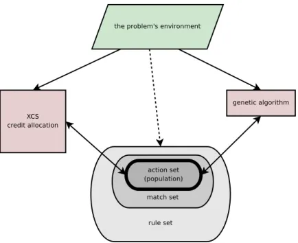
1.4.3. XCS. ZCS has many positive features, especially its simplicity and the benefits derived from its cooperative fitness sharing, but there are some notable drawbacks, primarily that it usually will not evolve a complete mapping of the environmental states and allowable actions to the possible rewards, often quickly selects local optima, and breeds across niches, as noted in [4]. These drawbacks led Wilson to heavily modify ZCS into what is called XCS [4]. In XCS, several of the deficiencies in ZCS are addressed. The basic structure of XCS is graphically illustrated in Figure 1.2.

In ZCS, the GA is run on the entire population, a panmictic approach [7, p. 155]. This is ineffective for most problems, so in XCS the GA was run only in the current match set at the time step that the GA is run in the initial version of XCS, and only in the current action set at the time step that the GA is run in the later variants of XCS. We run the GA on the current action set in this work. This allows for a more accurate rule set to be evolved, since each niche is best viewed as its own sub-problem.

In ZCS, a rule is allowed to survive by the GA on the basis of its payoff. This is problematic, since it biases against rules early in a chain of events that are eventually profitable, and because rules that may be the most appropriate for an event might have a relatively low payoff. This caused ZCS to often fail to create a complete mapping and fail to evolve accurate generalizations. This is remedied in XCS by creating a fitness measure for the rules, separate from the predicted payoff, used by the GA.

Each rule r is now of the more complex form

r= (c,a,p,ε,F,exp,ts,as,n), (10) where:

• c is the condition matched by the rule r, comprised of elements from some alphabet such as{0,1,#}, where # is the matching symbol, matching both 0 and 1.

• a is the action that the rule r recommends. • p is the predicted payoff.

• ε is an estimate of the prediction error.

• F is the fitness used by the GA. It is vital that the fitness used by the GA is a measure of the accuracy of the rule, and not a measure of the magnitude of the rule, where the

Figure 1.2. XCS’s basic structure

magnitude of a rule is how active that rule is in relation to the rest of the rules in the rule set, since a rule with greater magnitude but lower accuracy can be a detriment to the system. For example, a rule that always matched every situation (all #’s in the condition) but only accurately predicted 51% of the situations would have high magnitude but low accuracy.

• exp is the experience of the rule, a count of the number of times since this classifier’s creation that it has belonged to the action set.

• ts is a time stamp of the last occurrence of a call to the GA in an action set that this classifier was a part of, as the generational number.

• as is an estimate of the average action set size this classifier has belonged to.

• n is the numerosity of this macro-classifier. This is how many traditional micro-classifiers this macro-classifier represents. Groups of entirely identical normal clas-sifiers (the micro-clasclas-sifiers) are subsumed into macro-clasclas-sifiers instead of being al-lowed to exist separately within the rule set; this serves solely as a computational

time-saver. Therefore the only difference between a normal classifier (a micro-classifier) and a macro-classifier is the presence of the numerosity, which is a count of how many micro-classifiers that specific macro-classifier represents.

1.4.4. XCSR. Wilson extended his concept of XCS with XCSR in [5]. Classifier systems had typically taken strings from some small alphabet, often binary, as input until then even though many real-world problems have input from the environment of the form

Rn _{for some order n∈}Z_{,n>0. Wilson’s XCSR allows XCS to operate on just such an}

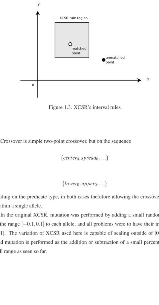
input. XCSR is identical to normal XCS with the exception of the input interface, the nature of the predicates, the mutation operator, and the details of covering. The basic structure of an XCSR rule is graphically illustrated in Figure 1.3.

Originally the predicates in XCSR were intervals of the form

intervali={centeri,spreadi}, (11)

such that an environmental input xiwas matched by intervaliif and only if

centeri−spreadi≤xi≤centeri+spreadi, (12)

but this was discovered to induce a bias [8], so the representation was eventually changed to be

intervali={loweri,upperi}, (13)

where now xiis matched by intervaliif and only if

loweri≤xi≤upperi. (14)

Figure 1.3. XCSR’s interval rules

Crossover is simple two-point crossover, but on the sequence

{center0,spread0, . . .} (15)

or

{lower0,upper0, . . .} (16)

depending on the predicate type, in both cases therefore allowing the crossover points to fall within a single allele.

In the original XCSR, mutation was performed by adding a small random quantity from the range[−0.1,0.1]to each allele, and all problems were to have their input scaled to [0,1]. The variation of XCSR used here is capable of scaling outside of [0.0,1.0], so instead mutation is performed as the addition or subtraction of a small percentage of the overall range as seen so far.

2. TIME SERIES PREDICTION

2.1. ARIMA AND OTHER STATISTICAL METHODS

ARIMA, the autoregressive integrated moving average, is a common and very power-ful statistical method often used in econometric models that can help forecast and estimate what is going to happen in the future. The ARIMA time series analysis uses lags and shifts in the historical data to uncover patterns (e.g., moving averages, seasonality) and predict the future [9]. The ARIMA model was first developed in the late 1960s but was not sys-temized until the work of Box and Jenkins in 1976 [10]. ARIMA can be more complex to use than other statistical forecasting techniques, although when implemented properly can be quite powerful and flexible. ARIMA is a method for determining two things:

1. how much of the past should be used to predict the next observation (length of weights) and

2. the values of the weights.

Three common models of time series data are autoregressive (AR) models, the in-tegrated (I) models, and the moving average (MA) models. These three classes depend linearly on previous data points and are combined in the autoregressive integrated moving average (ARIMA) model. A model of this form is referred to as an ARIMA(p,d,q)model where p,d,q∈N∗_{. The order of the autoregressive part is p, the order of the integrated part}

is d, and the order of the moving average part is q. Given a time series of data Xt (where t is integer valued and the Xt are real numbers) then an ARIMA(p,d,q)model is given by

1− p

∑

∑

where L is the lag operator,φ are the parameters of the autoregressive part of the model,θ are the parameters of the moving average part, d∈N∗ _{(if instead we have d=0 then this}

model is equivalent to an ARMA model), and theεt are error terms. The error termsεt are generally assumed to be independent and identically distributed variables sampled from a

normal distribution with zero mean:εt∼N(0,σ2)whereσ2is the variance. ARIMA mod-els are commonly used for predicting and analyzing simpler time series. They have been used on the stock market, but are generally viewed only as an indicator, not a predictive tool, due to the complexity of the market and because of their need for accurate knowledge about the time series itself. It is for similar reasons that most traditional statistical methods fail to be of any real use in this task.

For example y(t) =y(t−3) 3 + y(t−2) 3 + y(t−1) 3 (18)

is a potential ARIMA model; another potential ARIMA model is

y(t) =y(t−3) 6 + 4y(t−2) 6 + y(t−1) 6 . (19)

The correct ARIMA model requires identification of the right number of lags and the coef-ficients that should be used. ARIMA model identification uses autoregressions to identify the underling model. Care must be taken to robustly identify and estimate parameters as outliers (pulses, level shifts, local time trends) can wreak havoc.

2.2. ARTIFICIAL NEURAL NETWORKS

An artificial neural network is a graph of connected processing elements called neu-rons which can exhibit complex global behavior as determined by the connections between the neurons and their parameters. This technique was originally inspired by the examina-tion of the central nervous systems of living creatures, most notably that of humans, the most significant information processing system found in nature. While a neural network is not adaptive itself, most practical examples use algorithms designed to alter the weights of the connections in the network to produce a desired signal flow. These networks are also similar to their biological counterparts in that their functions are performed collectively in parallel by the entire network, with no clear delineation of sub-tasks to which various units are assigned. Modern artificial neural networks often abandon much of this for a more practical approach based on statistics and signal processing [11]. There have been many attempts to predict financial time series with artificial neural networks [12, 13], and there have even been somewhat successful results using genetic algorithms to evolve the weights for neural networks [14, 15]. However, there is one main drawback that comes with the

use of artificial neural networks. There is no easy way to translate the neural network that has been produced into an understandable set of rules describing its innate knowledge: the information is effectively trapped in the weights on the neurons. Extracting useful rules from ANN’s is a challenging field unto itself [16].

2.3. NON-LCS EVOLUTIONARY APPROACHES

There have been attempts at using evolutionary approaches other than LCS’s to pre-dict and analyze markets and other time series, ranging from the simplistic to the very complex. In [17], traditional genetic algorithms were used to optimize the exact numbers to be used in traditional technical analysis. In [18], traditional genetic algorithms were again used, but this time in optimizing the rule sets for candlestick-style analysis; this out-performed a random trader. In [19], a simplified variant on the concept of genetic program-ming, coded in C++, was used to develop trading rules for six stocks, and they managed to return better results than both the market and a naive trader. However, the innate chal-lenges of the real market have lead many researchers to resort to simulated markets, whose simplicity can make fundamental discoveries about economic theory sometimes less chal-lenging to achieve; a small survey of these sorts of markets can be found in [20].

2.4. LCS-BASED APPROACHES

There have been a few attempts at using LCS’s to analyze and predict financial mar-kets. We will highlight a few derived from XCS here, since the system presented here is also derived from XCS.

2.4.1. XCS. A predictive system lacking a memory component is almost com-pletely useless in attempting to model a highly interdependent nonlinear multivariate time series such as the stock market with any hope of utility; none the less, it has been attempted. One of the more notable attempts at this is described in [21], in which an XCS was used to predict the correct trading action for a stock on consecutive trading days. Later work by Schulenburg and Ross in [22] does show some promise: they utilize the opinions of a large host of simulated traders in order to make a decision. This would yield in the gen-eral vicinity of 9%p.a. returns: not spectacular or applicable to real-world trading, but respectable.

2.4.2. XCSF. In [23] Wilson outlined an extension to XCS for the approximation of functions, called XCSF, which attempts to learn a function of the form y= f(x), where y∈R_{, |x|=n, and xi∈}Z_{∀xi∈x. A classifier consists of n interval predicates of the form} inti= (li,ui) and matches an input x if and only if li≤xi≤ui∀i∈N. Classical two-point crossover is employed, but where crossover may occur in-between the alleles or at the ends of the prediction, although the action is not involved in the crossover process. A covering classifier is generated for a situation x by forming the lithrough subtracting from xi some random integer from [0,r0], and forming ui by adding some other random integer from [0,r0]to xi, both limited to a maximum range of possible input, where r0is a parameter. A rule r1 can subsume a rule r2 if and only if l1_i ≤l_i2∧u2_i ≤u1_i∀i. While this could possibly be used to predict some very simplistic time series data, function approximation often does not perform very well in real-world problems, as is well-known in reinforcement learning literature [24, 25], and this drawback of XCSF (and similar approaches) is explicitly ac-knowledged in [26]. This would be most definitely true of a system as complex as the stock market, which cannot be easily and usefully mapped to any polynomial.

3. APPROACH AND DESIGN OF THE TIME SERIES CLASSIFIER

3.1. FUNDAMENTAL OPERATIONS

Our representation of a time series and our approach to their evolutionary methods requires us to be capable of generating multi-dimensional raster paths, where a raster path is a one-dimensional path through a raster space. This is so that we can run raster paths through a raster space of data, a discrete sampling of data. A raster space is one that is representable by Z_a×Z_{b× · · · ×}Z_{z. In other words, all of the dimensions are along sets}

of finite integers instead of the real numbers. A common example is raster imagery: a two-dimensional bitmap of size m×n can be viewed as a complete representation of the two-dimensional raster space ofZ_m×Z_{n. A multidimensional matrix can therefore fully}

represent these spaces, instead of merely being samplings of the real space, although we are using these raster spaces for sampling of real data in our approach. We form a useful sample of the data for further analysis and classification by TSC by generating paths through the data and it is these raster paths that the TSC actually classifies the situations with, not with the entire data set which is generally very large. We will now outline the basic operations we use to generate raster lines.

3.1.1. The Sort On Algorithm. This algorithm sorts a sequence s according to the ordering of another sequence t, and is outlined in Algorithm 3.1.

Input: A sequence s to be sorted.

Input: A sequence t upon which to sort s with. Input: A comparator c to sort with, typically>or<.

Require: |s|=n≤ |t|.

1. Construct a sequence u containing pairs of the form ui= (si,ti)as elements,|u|=n,

u= (u0, . . . ,un−1) = ((s0,t0), . . .,(sn−1,tn−1)). (20)

2. Sort u using the second elements as the key, using any normal sorting algorithm, giving

u′= (s′₀,t₀′), . . .,(s′_n−1,t_n′₋₁)

(21) where t₀′ ≤. . .≤t_n′₋₁if we are sorting in ascending order (with the<comparator).

3. return s′= s′₀, . . .,s′_n−1.

Algorithm 3.1. Sort on.

3.1.2. The Sort Order Algorithm. This algorithm returns the re-ordered indices of a sorted sequence, and is outlined in Algorithm 3.2. For example, if t={4,5,3,9}then the sorted ordering of t would be{3,1,0,2}since t3≥t1≥t0≥t2.

Input: A sequence t.

Input: A comparator c, usually<or>.

1. let n← |t|.

2. GenerateZ_{n= (0, . . . ,n−1).}

3. return The result of the sort on algorithm from §3.1 on s=Z_{n with t and the}

com-parator c.

Algorithm 3.2. Sort order.

3.1.3. Rasterized Linear Paths Through Arrays. Given an array A of rank r and dimensions d0× · · · ×dr−1, we wish to pull a one-dimensional list or vector v of values from the array, starting at position As0...sr−1 and finishing at position Af0...fr−1, following a

As an example consider the 4×6 array: A=        a b c d e f g h i j k l m n o p q r s t u v w x        .

3.1.3.1. A purely horizontal path. The linear path from A0 0 to A0 5 would be composed of the values

hA0 0,A0 1,A0 2,A0 3,A0 4,A0 5i and would be ha,b,c,d,e,fi as illustrated by A=        a⋆ b⋆ c⋆ d⋆ e⋆ f⋆ g h i j k l m n o p q r s t u v w x        .

3.1.3.2. A purely vertical path. The linear path from A0 0to A3 0 would be com-posed of the values

hA0 0,A1 0,A2 0,A3 0i and would be ha,g,m,si as illustrated by A=        a⋆ b c d e f g⋆ h i j k l m⋆ n o p q r s⋆ t u v w x        .

3.1.3.3. A traditional diagonal path. The linear path from A0 0 to A3 3would be composed of the values

and would be ha,h,o,vi as illustrated by A=        a⋆ b c d e f g h⋆ i j k l m n o⋆ p q r s t u v⋆ w x        .

3.1.3.4. Non-equal diagonal paths. The confusing part arises when we are deal-ing with diagonal paths with unequal steps. Consider the linear path from A0 0to A3 5. We end up with a stair-stepping path through the array:

(A0 0,A1 1,A2 1,A3 2,A4 2,A5 3) and would be (a,h,i,p,q,x) as illustrated by A=        a⋆ b c d e f g h⋆ i⋆ j k l m n o p⋆ q⋆ r s t u v w x⋆        .

3.1.3.5. The Raster Line Algorithm. This is the algorithm used to determine a linear raster path, and is outlined in Algorithm 3.3. It returns a list of points that follow the linear path from the starting point p to the ending point q. This is derived from the algorithm for raster conversion of a 3D line as described in [27]. This should work for any dimensionality.

Input: a starting point p and a final point q, both represented as lists. Require: |p|=|q| ∧pi∈N∀pi∈p∧qi∈N∀qi∈q.

1. if p=q then // This is a simple degenerate case.

2. return {p}, a list containing only one element, p.

3. let n← |p|=|q|be the dimensionality.

4. letδ ← {|p0−q0|, . . .,|pn−1−qn−1|},|δ|=n.

5. let o be the sorted ordering ofδ by>from the sort order algorithm in §3.2.

6. let p′and q′be p and q respectively, sorted according to o.

7. if p′₀≤q′₀then // We want the starting point to have the lower initial dimension.

8. Swap p′with q′.

9. letδ′←

|p′₀−q′₀|, . . .,|p′_n−1−q′_n−1| .

10. let s← sgn p′₀−q′₀, . . . ,sgn p′_n−1−q′_n−1, where sgn is the signum function.

11. let d ← {d1, . . . ,dn−1},|d|=n−1, the deciders, where di←2δ_i′−δ₀′∀di∈d.

12. let a← {a1, . . .,an−1},|a|=n−1, the if-increments, ai←2δ_i′∀ai∈a.

13. let b← {b1, . . .,bn−1},|b|=n−1, the else-increments, bi←2 δi′−δ0′

∀bi∈b.

14. let r ← {p′}, initializing the result of the algorithm, an ordered list of points.

15. let z← p′, initializing the current point.

16. while z0<q′₀do // After this, we have r={p′, . . .,q′}.

17. Increment z0by 1.

18. for all di∈d do

19. if di<0 then

20. increment diby ai.

21. else // In this case we have di≥0.

22. increment diby biand ziby si.

23. Push a duplicate of z to the back of r, so that now r={p′, . . . ,z}.

24. Reorder the coordinate of the points in r according to the original coordinate ordering forming r′by applying the inverse of o, which is o.

25. if we originally swapped the start and end points then

26. return the reverse of r′.

27. else

28. return r′.

Algorithm 3.3. Raster line.

3.1.4. List Slices. This function returns a slice from a one-dimensional list; that is, a modular subset of the list, and is outlined in Algorithm 3.4. For example, a 2-slice of the list{1,2,3,4,5,6,7,8,9}would be the list{1,3,5,7,9}.

Input: A list of elements l={l0,l1, . . . ,l|l|}.

Input: A positive rational slice size s.

1. Initialize the resulting list r←nil={}, initially empty.

2. Initialize the moving index i←0.

3. while i<|l|do

4. if i∈Z_then

5. Append lito the end of r.

6. i←i+s.

7. return r.

Algorithm 3.4. List slice.

3.2. DATA REPRESENTATION

This LCS is intended to operate on a multivariate time series. The data consists of a single temporal dimension, several positional dimensions, and a single dimension of type. This is represented as a linked list consisting of multidimensional arrays, where each element in the matrices is a structure. Each array of structures represents a single time step; the position in the list is the position in time. The fields of the structures are independent data. Thus, any specific value in the multivariate time series could be uniquely referenced in the form:

{t,x0, . . . ,xn−1,φ} (22) where t is the temporal position, x0, . . . ,xn−1 are the dimensional positions (for n dimen-sions), and φ is the field selector. It must hold that ∀xi∈N∗. The temporal position t specifies a time tcurrent−t, and it must also hold that t∈N0.

This representation can be simplified: the entries can be single elements instead of full structures, and the arrays themselves can even be reduced to single elements, reducing to a traditional one-dimensional time series, all using the same code. This is what is done in the examples here, and all tests were performed on one-dimensional time series, although each entry was a structure containing multiple related data. For our example of market analysis, t is the number of days from present time, and the fields are the opening price, closing price, high price, low price, adjusted closing price, and the volume of the trades for that particular stock at that particular time.

3.3. RULE REPRESENTATION

The representation of a single rule is a collection of predicates; each predicate must match the current situation for the rule to match the situation. A single predicate consists of an initial and a final position, each of the form

{t,x0, . . .,xn−1}, (23) a field selector φ, an operator ω, and a range pair consisting of a lower and upper bound

[l,u]. The field selector φ is to be a lexical closure taking only one argument, which is the structure at the position{t,x0, . . . ,xn−1}. If the structure is not a structure, but rather a single element, the only value that would usually make sense forφ would be an identity function: simple transformative functions would be acceptable otherwise. Any function that operates in a uniform manner, applied to a single entry, would be an acceptableφ. The operatorω is also a lexical closure, and is intended for classification purposes; allω’s must operate over a one-dimensional vector of data.

If we take the data along the straight line segment from the initial point A to the final point B, forming a vector d, we can then form d′by applyingφ to each element in d:

d_i′=φ(di)∀di∈d. (24)

The predicate is said to match the data if and only if

l≤ω d′≤u. (25)

When all of the predicates of the rule match, then the rule matches; the rule then recom-mends a particular classification or action.

3.4. MUTATION

The approach to mutation of the paths is to restrict the mutation of the line segment to the same line, only allowing the end points to move up or down along that line. In this method, the alteration of the line segment is minor, and therefore there is very little

change in the actual information held by the path. This is exactly the sort of effect we wish in mutation: small changes. By only allowing for smaller mutations we do not have the information stored in the rule itself destroyed completely, but instead it is just slightly modified.

◦ • • • •

The lower and upper values of the range are altered, but limited by a maximum mutation parameter, and also limited to ensure that the current situation maintains its current classi-fication under the classifier rule.

3.5. CROSSOVER

We use a marginally-modified form of one-point crossover. Consider viewing the environment condition of a rule as consisting of several predicates, each possessing an initial point A, a final point B, a lower bound l, an upper bound u, a fieldφ and an operation

ω. We could choose to view this as a list of the form

A0,B0,l0,u0,φ0,ω0, . . . ,Ap−1,Bp−1,lp−1,up−1,φp−1,ωp−1 (26) where p is the number of predicates contained in the rule. Apply one-point crossover on two lists of this form, but insure that both lists break the predicates in the same way.

3.6. LEARNING PARAMETERS

There are numerous parameters used in XCS, a few added by XCSR, and a few more still added here. Choosing their values wisely can be very important in some problem domains unfortunately. This subsection gives brief descriptions of the important parameters and specifies sensible default values for typical problems. It is important that any results described should also list the parameter settings used.

3.6.1. From XCS. These are the parameters that are present in XCS. As such, they are also present in XCSR and TSC.

3.6.1.1. General Parameters These are parameters related to the general opera-tion of XCS.

Maximum total numerosity. This is N in [28]. It specifies the maximum size of the

classifiers. This should be a positive integer, normally in the hundreds or at most the thousands.

Learning rate. This is β in [28]. It is used as the learning rate for the predicted payoff, prediction error estimate, GA fitness, and action set size estimate for the classifiers. This should be in the range [0.1,0.2] for most problems, and always in the range

[0,1).

Possible actions. This is A_{, the set of all of the possible actions that the classifier rules} may take for values of a.

3.6.1.2. Recalculating Fitness These parameters are used in XCS while recalcu-lating the fitness of the rules in the population.

Multiplier parameter. This isα in [28]. This is the multiplier used in recalculating the fitness of the classifiers in the update fitness algorithm from §3.7. It is usually around 0.1.

Equal error threshold. This isε0 in [28]. This is the threshold used in recalculating the fitness of the classifiers in the update fitness algorithm from §3.7 to decide if the errors are essentially the same. It is usually around 1% of theρ, the reward.

Power parameter. This isν in [28]. This is the exponent used in recalculating the fitness of the classifiers in the update fitness algorithm from §3.7. It is typically set to 5.

3.6.1.3. Multi-Step Specific These are parameters that are only used in multi-step problems.

Discount factor. This is γ in [28]. It is the discount factor used in multi-step problems when updating the classifier predictions. It is typically around 0.71.

3.6.1.4. GA Specific These parameters are only used by the GA within XCS.

GA Threshold. This is θGA in [28]. The GA is run whenever the average number of generations since the last time the GA was run is greater than this threshold. It is typically in the range[25,50], and should always be inN∗_.

Crossover probability. This is χ in [28]. It is the probability of applying the crossover operator while executing the GA. It is typically in the range[0.5,1.0].

Mutation probability. This is µ in [28]. It is the probability of applying the mutation operator while executing the GA. It is typically in the range[0.01,0.05].

Deletion threshold. This is θdel in [28]. It is the threshold for classifier deletion. If a classifier’s experience is greater than this parameter then it may be considered for deletion. It is typically 20.

Fitness fraction threshold. This is δ in [28]. It is the fraction of the mean fitness of the population below which the fitness of a classifier may be considered in its probability of deletion. It is typically around 0.1.

Initial fitness. This is FIin [28]. It is used as the initial value of the fitness used by the GA for the newly-created classifiers. It is typically only slightly more than zero.

3.6.1.5. Rule Set Specific These parameters deal with the rule set as a whole.

Minimum subsumption experience. This is θsub in [28]. The experience of a classifier must be greater than this threshold for it to subsume another classifier. It must hold thatθsub∈N∗, and typically we haveθsub≥20.

Covering probability. This is P#in [28]. It is the probability of using the covering element in a single attribute. It is typically around 0.33.

Initial prediction. This is pI in [28]. It is used as the initial value of the predicted payoff for the newly-created classifiers. This is typically slightly more than zero.

Initial prediction error. This is εI in [28]. It is used as the initial value of the estimated prediction error for the newly-created classifiers. It is typically only slightly more than zero.

Exploration probability. This is P_explr in [28]. It specifies the probability of exploration during the action selection phase. It is typically around 0.5.

Minimal number of actions. This isθmna in [28]. This should be in N, and is typically equal to the number of possible actions, so that complete covering will take place.

Maximum number of steps. This is the maximum number of steps that a multistep

prob-lem can spend in one trial. This variable is not mentioned in [28], but it is present in Butz’s XCS code written in the C programming language.

GA subsumption? This is doGASubsumption in [28]. It is a boolean parameter specifying

if the offspring are to be tested for possible logical subsumption by the parents. It is usually best to set this to true.

Action set subsumption? This is doActionSetSubsumption in [28]. It is a boolean

param-eter specifying if action sets are to be tested for subsuming classifiers. It is usually best to set this to true.

3.6.2. From XCSR. These are the learning parameters that are added to an XCS system by XCSR. Since our system derives from XCSR, we use these as well. The variables used here are slightly different from those in a traditional XCSR.

Problem range. This is a two-element list of the lower and upper values that the input is

expected to lie within. As the input violates this, this range is expanded automatically. As an example, if it is known for a specific problem that the input should always lie within the real-valued range[0,1], then this should be set to the list{0.0,1.0}.

Covering maximum. This is how large of a fraction of the range can be added to both

the lower and upper bounds combined in the covering. The current default value we are using is 0.1. Thus, if we wish to cover[0.3,0.5], which has a spread of 0.5−

0.3=0.2, the largest allowable spread would be(1+coveringmaximum)spread= (1+ 0.1)0.2=0.22.

Mutation maximum. This is how large of a fraction of the range may be added or

sub-tracted from the lower and upper bounds in the mutation method. The current default value we are using is 0.1. For example, if we are mutating a rule which matches the bounds[0.3,0.72], which has a spread of 0.72−0.3=0.42, we would have a max-imum change of 0.042, so our mutated rule would now match bounds determined randomly from [0.3±0.042,0.72±0.042], but enforced to be within the problem bounds.

Initial spread limit. This is s0in [5]. It is the maximum initial spread when a new predi-cate is created through the covering operator.

3.6.3. New in TSC. These parameters are introduced here in TSC.

Maximum environment condition length. This is how many predicates we may have at

the maximum in any individual classifier. It should always be a positive integer.

Maximum temporal mutation. This is the most that the temporal element of the

posi-tion may be randomly perturbed during the mutaposi-tion process. It should always be a positive integer.

Maximum position mutation. This is the most any dimensional element of a position

may be randomly perturbed during the mutation process. It should always be a posi-tive integer.

Valid operations. This is a list of all the valid operations for the classifier, the ω’s, a list of first-order lexical closures. A first-order lexical closure is, roughly speaking, a function and its associated scope. These ω’s each must be capable of operating on any arbitrary list of data extracted from the data set, and these lists of data are extracted by following the raster paths through the data.

Valid fields. This is the list of valid fields for the classifier, the φ’s, a list of first-order lexical closures. Theseφ’s must be capable of operating on a single time instance of the data.

Visible time range. This is the range in time that is visible to the classifiers. None of the

classifiers are allowed to look beyond this window. This also is generally how much of a history should be generated before the classifier system is allowed to start. This is a set interval.

3.7. TRIVIALLY MODIFIED ALGORITHMS

There are several algorithms from XCS and XCSR that are only slightly modified for our purposes from their original forms.

The Generate Match Set Algorithm. This is the GENERATE MATCH SET function in

[28]. The match set M contains all of the classifiers in the population P which match the current situation. After filling the match set with all pre-existing matching clas-sifiers, it repeatedly generates new covering classifiers until the minimum number of actions is satisfied.

The Select Action Algorithm. This is the same as in traditional XCS. There are two

meth-ods for selecting an action used here: either randomly, or the best action.

The Generate Action Set Algorithm. This is the GENERATE ACTION SET function in

[28]. It forms the action set A out of the match set M, all of the classifiers that match the selected action.

The Update Set Algorithm. This is the UPDATE SET function in [28]. It updates the

parameters for classifiers in the action set.

The Update Fitness Algorithm. This is the UPDATE FITNESS function in [28]. The

fit-ness of all of the classifiers in the action set are updated in a normalized manner.

The Run GA Algorithm. This is the RUN GA function in [28]. It runs a simple genetic

algorithm, not on the full population P, but instead only on the action set A, in order to induce niching.

The Select Offspring Algorithm. This is the SELECT OFFSPRING function in [28]. It

uses a roulette-wheel method of selection.

The Insert into the Population Algorithm. This is the INSERT IN POPULATION

algo-rithm in [28]. It is slightly more complex than just pushing the new classifier into the population list: we need to check to see if it is already present in the population. If it is, we must increment that classifier’s numerosity instead. For a new classifier r, find an r′∈P, with P being the entire population, such that r and r′are identical. If such an r′exists, increment r_n′; otherwise insert r into P.

The Delete from Population Algorithm. This is the same as the DELETE FROM POPU-LATION function in [28]. It decides which members of the population are suitable for deletion, allowing for niching, and then removes low-fitness individuals.

The Deletion Vote Algorithm. This is the same as the DELETION VOTE algorithm in

[28]. The deletion vote for a classifier r is dependent upon its action set size estimate. Let Faverage be the average fitness in the entire population. We want classifiers with sufficient experience and a significantly lower than average fitness than the rest of the population to be deleted before others. Expressed in terms of the TSC parameters as outlined in §3.6:

rexp>θdel

^rF

rn

<δFaverage. (27)

This then returns

rasrnFaverage rF rn = rasr_n2Faverage rF (28)

as the deletion vote for this classifier r; otherwise it returns rasrnas the deletion vote for this classifier r.

The Do Action Set Subsumption Algorithm. This is the DO ACTION SET SUBSUMP-TION function in [28]. The function chooses the subsumer from the most general classifiers capable of subsumption and then subsumes all possible classifiers in to the subsumer.

The Could Subsume? Predicate. We say that a specific classifier r is capable of

subsum-ing others if it has both sufficient accuracy and sufficient experience. That is, if the experience of the classifier is greater than the minimal subsumption experience threshold, and the prediction error of the classifier is less than the equal error thresh-old. In symbols:

rexp>θsub

^

r_ε <ε0. (29)

The Subsume? Predicate. This is called DOES SUBSUME in [28]. A classifier r1 sub-sumes another classifier r2if the following conditions are all met:

1. Their actions are identical: r1_a=r2_a.

2. The classifier r1 is capable of subsumption, as decided by the could subsume? predicate described in §3.7.

3. The classifier r1 is more general than the classifier r2, as decided by the more general? predicate described in §3.10.

3.8. THE MATCH? PREDICATE

This is based upon the algorithm called DOES MATCH in [28], but it has been gener-alized in order to suit our needs here. Assume a classifier r and a situationσ. In traditional learning classifiers,σ ∈ {f alse,true}which is usually represented {0,1}, and therefore it is only necessary to see if every element in the condition part of the classifier r, that is rc, is either equal to each other or a covering symbol in r:

rci=σi _ rci=# ∀i∈Z_{|rc|=|σ|. (30)}

For us, it is slightly more involved due to the more complex nature of the conditions used in the construction of the classifiers.

The match? predicate for ternary values. For ternary values as used in traditional

learn-ing classifiers, a ternary predicate t matches a situation element x when either t =x or t = #, the covering symbol. Similarly, a ternary predicate t matches a second ternary predicate u when t matches all of the situations matched by u; that is, when t=uW

t=#.

The match? predicate for ranges. For ranges as used in Wilson’s XCSR [5], a range

predicate r matches a situation x when that situation x lies within the lower and upper bounds specified by the range predicate, l≤x≤u.

The match? predicate for a time-series. If we take the data along the straight line

seg-ment from the initial point A to the final point B, forming a vector d, we can then form d′by applyingφ to each element in d:

d_i′=φ(di)∀di∈d. (31)

The predicate is said to match the data if and only if

When all of the predicates of the rule match, then the rule matches; the rule then recommends a particular classification or action.

Two situationsσ1andσ2match if every one of their elements match element-wise:

match?(σ1i,σ2i) =true∀i∈Z|σ1|=|σ2|. (33)

The match? predicate for classifiers and situations. A classifier r matches a situationσ

if r1and r2match, as decided by the match? predicate described in §3.8, and at least one of the elements of the classifier is more general in r1than in r2.

The match? predicate for classifiers. A classifier r1 matches another classifier r2 if the environment condition of r1matches the environment condition of the classifier r2.

3.9. THE GENERATE COVERING CLASSIFIER ALGORITHM

This is derived from the GENERATE COVERING CLASSIFIER function in [28]. It creates a classifier which matches the current situation. This is handled somewhat differ-ently in TSC than in XCS or in XCSR, and the method operates as described in Algo-rithm 3.5.

Input: a TSC instance.

1. let l be randomly chosen, 1≤l≤the maximum environment condition length.

2. let c, the condition←nil={}, an empty list.

3. let a, the action←a random element from the set of all possible actions that are not in the match set.

4. for l times do

5. push a covering predicate onto c

6. return a new classifier instance with environment condition c, action a, time stamp

set to the current number of situations, and the rest of the slots set to their defaults.

Algorithm 3.5. Generating covering classifiers.

3.10. THE MORE GENERAL? PREDICATE

The more general? predicate for a TSC predicate. This returns true only if the predicate p matches predicate q and if it is more general than it as well. Predicate p is more general than predicate q if and only if:

p matches q∧

lp<lq∨uq<up∨ pathqlies completely along pathp∧pathp6=pathq

.

The more general? predicate for classifiers. This is based upon the algorithm called IS MORE GENERAL in [28], but it has been generalized in order to suit our needs here. In traditional learning classifiers, it is only necessary to count the occurrences of the covering symbol, #, in order to determine which of two classifiers is more general: the one with the greater number of occurrences of it. For us it is slightly more in-volved due to the more complex nature of the conditions used in the construction of the classifiers. A classifier r1is more general than another classifier r2 if r1 and r2 match, as decided by the match? predicate described in §3.8, and at least one of the elements of the classifier is more general in r1than in r2.

4. EXPERIMENTAL RESULTS

4.1. THE NATURE OF A REALISTIC TIME SERIES

The primary difficulty experienced in testing was an unknown aspect of time series themselves. Originally the test problem was a very simple one-dimensional sine wave, with only a simple slope function for an operator, and with the classification task of deciding if the next point will be up or down from the current point. This appears as if it were a trivial problem, and indeed a high degree of accuracy can be achieved with only two very simple rules: if the previous point is below the current one then the next point will be above; otherwise the next point will be below the current point.

This approach will not work in general. There are several distinct types of time series, such as: up-trending, down-trending, steady, periodic, up-step, down-step, hills, and valleys. Real-world time series are comprised of several of the characteristics from each type, and any system that would be capable of operating on a real-world time series would need to be able to handle all of the different types simultaneously. The problem is that a simple slope operator is only capable of learning time series that are primarily linear, and a periodic time series such as the sine wave requires entirely different operators.

4.2. THE SIMPLISTIC INCREASING/DECREASING TESTS

The original test time series was a sine wave, which is a perfect example of a peri-odic function, but the simple slope operator is only capable of learning linear time series data. The new tests were designed with this in mind, and is actually a closer match to the appearance of real market data.

The first new test was simply a randomly chosen slope for a line, either upward or downward; the classification question is still whether or not the next point will be above or below the current one; this was very quickly optimally learned by the system.

In the second simple test, the series is randomly selected to be either upward or downward for a random number of time steps, with a randomly chosen slope, over and over again with completely different random elements each time. This was also very quickly optimally learned by the system.