Optimizing Expected Profit Under Flexible Allocation of Campaign Days and Budget for Management of Shopping Centers: A Machine Learning Approach

(1)

Optimizing Expected Profit Under Flexible Allocation of

Campaign Days and Budget for Management of

Shopping Centers: A Machine Learning Approach

Nora Sharkasi

Tokyo International University, International University of Japan

Corresponding Author: [email protected]

Jay Rajasekera

Institute of International Strategy, Tokyo International University

Ushio Sumita

Graduate School of International Management, International University of Japan

ABSTRACT

In retail businesses, a sales campaign is typically organized over segments of

consecutive days within a certain period so as to maximize total sales in that period.

It is also common to design a sales campaign so that good-sales-days of the

previous year would be designated as sales campaign days, with the expectation

that the campaign effect could further enhance the potential of good-sales-days.

Sharkasi, Sumita, and Yoshii (2015) showed that, contrary to these common

practices, expected total sales can be increased by reallocating sales campaign days

in a more flexible manner. Their paper, however, focused exclusively on expected

total sales without regard to expected profit and did not consider the sales

campaign budget. The purpose of the current paper is to fill this gap by

incorporating the sales campaign budget per day, where the expected total sales

would be increased as a concave function of the budget increment. Furthermore,

expected profit rather than total expected sales is optimized. Based on a real dataset

from a shopping center in Tokyo, this study shows that expected profit could be

increased considerably with no additional cost using the optimization approach.

(2)

International Journal of Business and Information

1. INTRODUCTION

A shopping center (denoted by SC, hereafter) has many stores within its

premises, providing a variety of services such as retail stores, restaurants, food

services, beauty salons, and travel agencies. The origins of today’s SCs can be

traced to three SCs in the United States: Country Club Plaza, which opened in 1922

in Kansas City, Kansas; Town and Country Shopping Center, which opened in

1948 in Columbus, Ohio; and North Gate Shopping Center, which opened in 1948

in Seattle, Washington. Since then, SCs have expanded rapidly all over the world.

According to Guinness Book of World Records, the largest SC in the world in terms

of total area is the Dubai Mall, located within downtown Dubai, UAE.

Construction took about four years. Now, the mall comprises 1,200 retail outlets

and more than 160 food and beverage stores. Dubai Mall also includes an aquarium,

an Olympic-size ice rink, and a 22-screen Cineplex. The store mix of many

regional and national SCs are more or less similar (Burns & Warren, 1995;

Wakefield & Baker, 1998).

The competitive advantage of SCs over individual, independent retail stores is

that they offer a variety of stores and services in one place for the convenience of

consumers. They can provide cost-performance efficiency for their business

partners by allowing them to share parking lots, loading and unloading depots, and

other related facilities. Today, however, SCs operate in an increasingly competitive

environment characterized by overcapacity and a declining number of customers

(Shim & Eastlick, 1998; LeHew & Fairhurst, 2000).

At the time of building a new SC, the decision about its location and size would

be crucial to gain a competitive advantage over other existing SCs (Ahmadi-Javid,

et al., 2018; Eckert, et al., 2015; Yu, et al., 2007; Christaller, 1966; Weber, 1969;

Eppli & Benjamin, 1994). Other important decisions include selection of tenant

stores and choice of so-called “anchor” stores. Once these decisions are made, it

(3)

it then becomes important to manage available resources wisely to enhance

profitability. Knowing how to organize sales promotions efficiently would be the

key to success. This paper addresses this challenging issue.

In the era of big data analysis, it is now possible to collect massive amounts

of data from tenants of an SC via a point-of-sales (POS) system so as to assess the

effects of promotional activities. An extensive literature exists for analyzing

consumer purchasing behavior based on POS data, including studies by Eugene

(1997), Yada et al. (2006), Taguchi (2010), and Ishigaki et al. (2011), to name only

a few. Little research has been done, however, on how to use POS data to manage

SC business. Kumar, Shah, and Venkatesan (2006) addressed issues on how to

evaluate customer lifetime value at the individual customer level so as to maximize

SC profitability. An interesting case study of an SC in Iran was examined by

Balaghar, Majidazar, and Niromand (2012), who assessed the effectiveness of

promotional tools such as advertisement, sales promotion, public relations, and

direct selling.

The topic of profit optimization in retail business can be approached from

various perspectives. Retailers aim to maximize profit by considering potential

revenues, purchase costs, diminishing profits for products, and opportunity costs

for unfulfilled demand. Optimal profit may also be approached through optimal

traffic assignment, cost structure, capacity maximization, and property structure.

In recent studies, models were jointly developed to optimize decisions for product

prices, display orientations, and shelf-space locations in a product category to

optimize profits (e.g., Sun, et al., 2018; Hubner, et al., 2016; Katsifou, et al., 2014;

Murray, et al., 2010).

A mixed-integer programming and nonlinear optimization model

incorporating both essential in-store costs and space and cross-elasticities for profit

maximization was developed by Irion, et al. (2012). In a recent paper, Hubner and

Schaal (2017) developed a decision model integrating assortment and shelf-space

planning by considering stochastic and space-elastic demand, and

(4)

results even for large-scale problems. Models incorporating optimal product

assortments, along with promotional efforts and inventory and pricing models,

have been discussed by a wide array of researchers (Rambha, et al., 2018; Hubner

& Schaal, 2017; Heuvel & Wagelmans, 2017; Hubner, et al., 2016; Chapados, et

al., 2014; Katsifou, et al., 2014; Wang & Li, 2012; Bhattacharjeea & Rameshb,

2000). Another stream of literature focuses on optimal scheduling such as

workforce shift scheduling and pricing in the retail sector for profit optimization

(Yong & Li, 2017; Kabak, et al., 2008).

A typical management arrangement of an SC-wide promotion is that retail

outlets provide the promotion for an event in conjunction with mall management.

Based on the analysis of a survey and three months of actual data, Parsons (2003)

found that SC-wide promotions are the most preferred. Furthermore, a

combination of general entertainment and price-based promotions were found to

be strong drivers for visits and spending by consumers, whereas community and

educational promotions enhanced the traffic of non-customers. An SC-wide sales

campaign is typically organized over segments of consecutive days. It is common

to design a sales campaign in such a way that strong-sales-days of the previous

year would be designated as sales campaign days for the current year. This is done

because of the expectation that the campaign effect could further enhance the

potential for strong-sales-days.

In the original paper by Sharkasi, Sumita, and Yoshii (2015), a mathematical

model was developed for maximizing the expected total revenue in the SC by

reconfiguring how to schedule sales campaign days over a future period. The paper

showed that, contrary to the common practices described above, it could be more

effective to schedule sales campaign days over weak-sales-days. This finding

implies that the campaign effect to enhance expected total sales over

(5)

The purpose of the current paper is to expand on the original paper by

Sharkasi, Sumita, and Yoshii (2015) by considering the problem of optimizing

total expected profit rather than total expected sales, subject to a campaign budget.

This paper is structured in five sections. Section 2 focuses on data description

and cleansing; Section 3 discusses problem formulation; Section 4 presents the

numerical results of the study; and Section 5 provides study conclusions

2. DATA DESCRIPTION AND CLEANSING

In this study, we work on a set of real data obtained from an SC in Tokyo for

Winter 2010 (December 2009 and January and February 2010) and for Winter

2011 (December 2010 and January and February 2011). The set of days in Winter

2010 is denoted by 𝐷𝐷_{𝐿𝐿𝐿𝐿} , where LD stands for Learning Data. Similarly,

𝐷𝐷𝑇𝑇𝐿𝐿denotes the set of days in Winter 2011, to be used as Testing Data. Since the data structure of Winter 2011 is identical to that of Winter 2010, we describe the

data structure only for day𝑖𝑖 ∈ 𝐷𝐷_{𝐿𝐿𝐿𝐿}. A record for day 𝑖𝑖 ∈ 𝐷𝐷_{𝐿𝐿𝐿𝐿}consists of the following elements.

𝐼𝐼𝐶𝐶𝐶𝐶𝐶𝐶𝐶𝐶(𝑖𝑖): the campaign flag indicating whether the 𝑖𝑖-th day was under a sales campaign

(𝐼𝐼_{𝐶𝐶𝐶𝐶𝐶𝐶𝐶𝐶}(𝑖𝑖)=1) or not (𝐼𝐼_{𝐶𝐶𝐶𝐶𝐶𝐶𝐶𝐶}(𝑖𝑖)=0)

𝑠𝑠(𝑖𝑖): the total sales of the𝑖𝑖-th day in Japanese yen for the entire SC (2.1)

𝑡𝑡(𝑖𝑖): the number of purchase transactions of the 𝑖𝑖-th day for the entire SC It should be noted that, in the actual practice of the SC represented by the given

dataset, two separate price-based promotional campaigns were organized in both

(6)

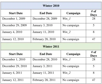
Table 1 shows the organization of the sales campaign days in Winter 2010 and

Winter 2011. We note that December and January each have 31 days, whereas

February has 28 days in both Winter 2010 and Winter 2011. The number of

campaign days in each winter totals 36.

Table 1

Number of Sales Campaign Days During Winter 2010 and Winter 2011 (As Indicated by Shopping Center)

Winter 2010

Start Date End Date Campaign # of Days

December 1, 2009 December 28, 2009 Win_1 28 December 29, 2009 January 3, 2010 No campaign 5 January 4, 2010 January 11, 2010 Win_2 8 January 12, 2010 February 28, 2010 No campaign 47

Winter 2011

Start Date End Date Campaign # of Days

December 1, 2010 December 28, 2010 Win_1 28 December 29, 2010 January 3, 2011 No campaign 5 January 4, 2011 January 11, 2011 Win_2 8 January 12, 2011 February 28, 2011 No campaign 47

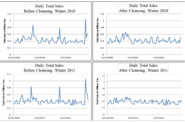
Throughout each year, the administration of the SC organizes some activities

or special events to attract more visitors. Consequently, these activities may result

in outliers in 𝑠𝑠(𝑖𝑖) and𝑡𝑡(𝑖𝑖). More specifically, let 𝜇𝜇_𝑠𝑠 and 𝜎𝜎_𝑠𝑠 be the mean and the standard deviation of the total sales over the winter period under consideration,

(7)

𝑠𝑠(𝑖𝑖) is an outlier ⟺ 𝑠𝑠(𝑖𝑖)≥ 𝜇𝜇_𝑆𝑆+ 2 𝜎𝜎_𝑆𝑆

𝑡𝑡(𝑖𝑖) is an outlier ⟺ 𝑡𝑡(𝑖𝑖)≥ 𝜇𝜇_𝑇𝑇+ 2 𝜎𝜎_𝑇𝑇

Let 𝜇𝜇_𝑆𝑆_:¬_𝑜𝑜 and 𝜇𝜇_𝑆𝑆_:_𝑜𝑜 be the average total sales of non-outlier days and that of outlier days, respectively. 𝜇𝜇_𝑇𝑇_:¬_𝑜𝑜 and 𝜇𝜇_𝑇𝑇_:_𝑜𝑜 are defined similarly. If 𝑠𝑠(𝑖𝑖) and𝑡𝑡(𝑖𝑖) are judged to be outliers, they are adjusted according to this formula:

𝑠𝑠(𝑖𝑖) ← 𝑠𝑠(𝑖𝑖) × 𝜇𝜇𝑆𝑆:¬𝑜𝑜/ 𝜇𝜇𝑆𝑆:𝑜𝑜 ; 𝑡𝑡(𝑖𝑖) ← 𝑡𝑡(𝑖𝑖) × 𝜇𝜇𝑇𝑇:¬𝑜𝑜/ 𝜇𝜇𝑇𝑇:𝑜𝑜 (2.2) Outliers may also result for other reasons. For example, a store in the SC under

study provides facilities for cultural classes; e.g., flower arrangement and piano

lessons. Monthly fees for such classes are paid on a fixed date of the month,

generating outliers in total sales. Outliers of this sort are adjusted by eliminating

the corresponding total sales and purchase transactions rather than using formula

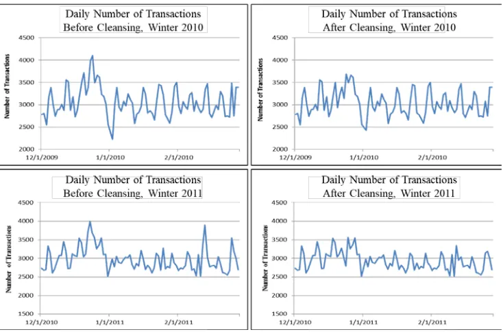
(2.2). Figure 1 shows the effect of cleansing all outliers in 𝑠𝑠(𝑖𝑖) for Winter 2010 and Winter 2011. The counterparts for 𝑡𝑡(𝑖𝑖) are depicted in Figure 2.

(8)

Figure 2. Purchase Transactions Before and After Cleansing, Winter 2010 and 2011

3. PROBLEM FORMULATION

In this section, we formulate the problem of determining the optimal

allocation of campaign days and the campaign budget so as to maximize expected

profit by expanding the mathematical model of Sharkasi, Sumita, and Yoshii

(2015). Here, a promotional campaign is organized so as to maximize the expected

profit over a given period of M days, subject to the number of campaign days being

N and the campaign budget𝐵𝐵_{𝐶𝐶𝑀𝑀𝑀𝑀}. A machine learning technique is used, with 𝐷𝐷_{𝐿𝐿𝐿𝐿} and 𝐷𝐷_{𝑇𝑇𝐿𝐿}as a set of Learning Data and a set of Testing Data, respectively. The total sales and the total number of purchase transactions for day𝑖𝑖 ∈ 𝐷𝐷_{𝐿𝐿𝐿𝐿} are denoted by𝑠𝑠_{𝐿𝐿𝐿𝐿}(𝑖𝑖) and𝑡𝑡_{𝐿𝐿𝐿𝐿}(𝑖𝑖), respectively. For day𝑗𝑗 ∈ 𝐷𝐷_{𝑇𝑇𝐿𝐿}, 𝑠𝑠_{𝑇𝑇𝐿𝐿}(𝑗𝑗) and𝑡𝑡_{𝑇𝑇𝐿𝐿}(𝑗𝑗) are defined similarly. The systematic approach used in this paper is structured in

(9)

3.1. Step I: Defining the Indicator Function of a Good-Sales-Day (GSD)

We begin our study by introducing the indicator function for a good-sales-day

(GSD). This function is a composite of the key performance measures of

promotional campaigns in shopping centers as guided by the literature; that is, the

total sales 𝑠𝑠_{𝐿𝐿𝐿𝐿}(𝑖𝑖) and the total number of purchase transactions 𝑡𝑡_{𝐿𝐿𝐿𝐿}(𝑖𝑖) at the end of business day𝑖𝑖. All days in 𝐷𝐷_{𝐿𝐿𝐿𝐿} are first placed in a descending order of 𝑠𝑠_{𝐿𝐿𝐿𝐿}(𝑖𝑖) and𝑡𝑡_{𝐿𝐿𝐿𝐿}(𝑖𝑖), separately. The percentile points in𝑠𝑠_{𝐿𝐿𝐿𝐿}(𝑖𝑖) and𝑡𝑡_{𝐿𝐿𝐿𝐿}(𝑖𝑖) are then marked, which we denote as 𝑆𝑆₀ and𝑇𝑇₀ , respectively. Table 2 summarizes these values obtained from the real data for Winter 2010 (𝐿𝐿𝐷𝐷) at different percentile points.

Table 2

Values for Total Sales and Number of Purchase Transactions, Winter 2010 (LD)

Percentile Total Sales in Billions

(𝑆𝑆₀)

Purchase Transactions

(𝑇𝑇₀)

Percentile Total Sales in Billions

(𝑆𝑆₀)

Purchase Transactions

(𝑇𝑇₀)

10% ¥ 5.517 3,502 60% ¥ 4.021 2,946

20% ¥ 5.187 3,391 70% ¥ 3.876 2,870

30% ¥ 4.671 3,233 80% ¥ 3.591 2,803

40% ¥ 4.511 3,140 90% ¥ 3.459 2,733

50% ¥ 4.226 3,014 100% ¥ 3.093 2,227

Using the thresholds 𝑆𝑆₀ and 𝑇𝑇₀ , the indicator function 𝐼𝐼_{𝐺𝐺𝐺𝐺𝐺𝐺𝐿𝐿}_:_𝑆𝑆₀_𝑇𝑇₀(𝑖𝑖) for𝑖𝑖 ∈ 𝐷𝐷_{𝐿𝐿𝐿𝐿} can be defined as

𝐼𝐼𝐺𝐺𝐺𝐺𝐺𝐺𝐿𝐿:𝑆𝑆0𝑇𝑇0(𝑖𝑖) =�1 , 𝑖𝑖𝑖𝑖𝑠𝑠𝐿𝐿𝐿𝐿≥ 𝑆𝑆0𝑎𝑎𝑊𝑊𝑎𝑎 𝑡𝑡𝐿𝐿𝐿𝐿

(𝑖𝑖)≥ 𝑇𝑇0 ,

0 , 𝑒𝑒𝑒𝑒𝑠𝑠𝑒𝑒 (3.1) where day 𝑖𝑖 is considered to be a good-sales-day (GSD) if 𝐼𝐼_{𝐺𝐺𝐺𝐺𝐺𝐺𝐿𝐿}_:_𝑆𝑆₀_𝑇𝑇₀(𝑖𝑖) = 1.

The numerical thresholds 𝑆𝑆₀ and 𝑇𝑇₀ obtained from the learning data LD are used to identify GSDs in the testing data TD so that 𝐼𝐼_{𝐺𝐺𝐺𝐺𝐺𝐺𝐿𝐿}_:_𝑆𝑆₀_𝑇𝑇₀(𝑗𝑗) can be defined similarly for𝑗𝑗 ∈ 𝐷𝐷_{𝑇𝑇𝐿𝐿}. As shown in Table 2, the values of 𝑆𝑆₀ and 𝑇𝑇₀ depend on which percentile is chosen. In the subsequent steps, a systematic approach is

(10)

International Journal of Business and Information 3.2. Step II: Using Logistic Regression and Confusion Matrix for

Appropriate Segmentation of GSD

Given the indicator function for sales campaign days, 𝐼𝐼_{𝐶𝐶𝐶𝐶𝐶𝐶𝐶𝐶}(𝑖𝑖) for 𝑖𝑖 ∈ 𝐷𝐷_{𝐿𝐿𝐿𝐿} as defined in equation (2.1), a logistic regression model is developed to estimate

the likelihood,𝜌𝜌_{𝐺𝐺𝐺𝐺𝐺𝐺𝐿𝐿}(𝑗𝑗) of whether day𝑗𝑗 ∈ 𝐷𝐷_{𝑇𝑇𝐿𝐿}in the future winter period is a GSD. For this purpose, we consider the set of explanatory variables given in

Table 3.

Following the standard procedure for eliminating multi-collinearity, the

correlation structure of these explanatory variables is given in Table 4. In this case,

it happened that the correlation of every pair is less than 0.5 and no variables are

eliminated because of multi-collinearity.

A logistic regression model is developed for estimating the likelihood,

𝜌𝜌𝐺𝐺𝐺𝐺𝐺𝐺𝐿𝐿(𝑗𝑗), of whether or not day 𝑗𝑗 in the future winter period is a GSD based on LD. Namely, from a set of the explanatory variables 𝑥𝑥_𝑘𝑘 (𝑖𝑖) for 𝑖𝑖 ∈ 𝐷𝐷_{𝐿𝐿𝐿𝐿} and 𝑘𝑘= 1,⋯,𝐾𝐾 , let 𝑥𝑥(𝑖𝑖) = [𝑥𝑥₁(𝑖𝑖),⋯,𝑥𝑥_𝑘𝑘(𝑖𝑖)] , and 𝛽𝛽= [𝛽𝛽₀,𝛽𝛽₁,⋯,𝛽𝛽_𝐾𝐾] . We define 𝑟𝑟 �𝑥𝑥(𝑖𝑖),𝛽𝛽� by

𝑟𝑟 �𝑥𝑥(𝑖𝑖),𝛽𝛽�= 𝛽𝛽0+ � 𝛽𝛽𝑘𝑘∙ 𝑥𝑥𝑘𝑘 (𝑖𝑖) 𝐾𝐾

𝑘𝑘=1

. (3.2)

The corresponding logistic regression model then yields the optimal

coefficient vector 𝛽𝛽∗, given by

𝛽𝛽∗_{= arg min}

𝛽𝛽 � �𝐼𝐼𝐺𝐺𝐺𝐺𝐺𝐺𝐿𝐿:𝑆𝑆0𝑇𝑇0(𝑖𝑖)−

𝑒𝑒𝑟𝑟(𝑀𝑀(𝑖𝑖), 𝛽𝛽)

1 +𝑒𝑒𝑟𝑟(𝑀𝑀(𝑖𝑖), 𝛽𝛽)�

2

𝑖𝑖∈𝐿𝐿𝐿𝐿𝐿𝐿

(11)

If 𝑥𝑥(𝑗𝑗) of day 𝑗𝑗 in the future winter period is known, equation (3.3) enables

one to assess the likelihood of day 𝑗𝑗 being a GSD. This measure, denoted

by𝜌𝜌_{𝐺𝐺𝐺𝐺𝐺𝐺𝐿𝐿}(𝑗𝑗), can be computed as

𝜌𝜌𝐺𝐺𝐺𝐺𝐺𝐺𝐿𝐿(𝑗𝑗) = 𝑒𝑒

𝑟𝑟(𝑀𝑀(𝑗𝑗), 𝛽𝛽∗₎

1 +𝑒𝑒𝑟𝑟(𝑀𝑀(𝑗𝑗), 𝛽𝛽∗) . (3.4)

By specifying a threshold level 𝜌𝜌_{𝐺𝐺𝐺𝐺𝐺𝐺𝐿𝐿}, equation (3.4) then enables one to determine whether or not day 𝑗𝑗 is judged to be a GSD. More specifically, we define

𝐼𝐼̂𝐺𝐺𝐺𝐺𝐺𝐺𝐿𝐿(𝑗𝑗) =� 1 , _{0 ,}𝑖𝑖𝑖𝑖𝜌𝜌𝐺𝐺𝐺𝐺𝐺𝐺𝐿𝐿_{𝑒𝑒𝑒𝑒𝑠𝑠𝑒𝑒}(𝑗𝑗)≥ 𝜌𝜌𝐺𝐺𝐺𝐺𝐺𝐺𝐿𝐿 . (3.5)

In order to determine the threshold level 𝜌𝜌_{𝐺𝐺𝐺𝐺𝐺𝐺𝐿𝐿}, we use the confusion matrix obtained, as shown in Table 5. This approach is widely used in the area of

(12)

Table 3

Definitions of Explanatory Variables Considered for Logistic Regression

Label Description

𝑾𝑾𝑾𝑾𝑾𝑾𝑾𝑾_𝑾𝑾(𝒊𝒊),

k=1, 2, 3, 4 Each month has four weeks, labeled as: Week_1, Week_2, Week_3, _and_{Week_4. Any week consists of seven days, where Week_1}

starts from the first day of the month. Week_4 may include extra days until the end of the month. Week_k(𝑖𝑖) =1 if day 𝑖𝑖 belongs to Week_k; and 0, otherwise.

𝑾𝑾𝑾𝑾𝑾𝑾𝑾𝑾𝑾𝑾𝑾𝑾𝑾𝑾_𝑾𝑾(𝒊𝒊),

k= 1 ,⋯ ,5 Weekday_𝑘𝑘 (𝑖𝑖) takes the value of 1 when day 𝑖𝑖 in Week_k is a

weekday; and 0 otherwise. Each week has five weekdays, Mon, Tue, Wed, Thu, and Fri, labeled as Weekday_1, Weekday_2, Weekday_3, Weekday_4, and Weekday_5, respectively.

𝑾𝑾𝑾𝑾𝑾𝑾𝑾𝑾𝑾𝑾𝑾𝑾𝑾𝑾_𝑾𝑾(𝒊𝒊), k= 1 , 2 _{𝑊𝑊𝑒𝑒𝑒𝑒𝑘𝑘𝑒𝑒𝑊𝑊𝑎𝑎}_{_}_𝑘𝑘₍_𝑖𝑖₎ takes the value of 1 when day𝑖𝑖 in Week_k is Saturday or Sunday; and 0 otherwise.

𝑵𝑵𝑾𝑾𝑵𝑵𝒊𝒊𝑵𝑵𝑾𝑾𝑾𝑾𝑵𝑵_𝑯𝑯𝑵𝑵𝑵𝑵𝒊𝒊𝑾𝑾𝑾𝑾𝑾𝑾(𝒊𝒊) This binary flag indicates that day 𝑖𝑖 in Week k is an official national holiday in Japan.

𝑵𝑵𝑵𝑵𝑾𝑾_𝑾𝑾𝑾𝑾𝑵𝑵𝒊𝒊𝑵𝑵𝑾𝑾𝑾𝑾𝑵𝑵_𝑯𝑯𝑵𝑵𝑵𝑵𝒊𝒊𝑾𝑾𝑾𝑾𝑾𝑾(𝒊𝒊) This binary flag indicates that day 𝑖𝑖 is not an official national holiday but is likely to be very passive in business in Japan; e.g., December 28, 29, 30, and 31 when offices are typically closed.

Win_1(𝒊𝒊) _{This binary variable takes the value of 1 if day}_𝑖𝑖_{is under a sales} campaign in December; and 0 otherwise.

Win_2(𝒊𝒊) _{This binary variable takes the value of 1 if day}_𝑖𝑖_{is under a sales} campaign in January or February; and 0 otherwise.

LY_Transactions(𝒊𝒊) _{This binary variable takes the value of 1 if the number of}

transactions of day 𝑖𝑖 of the last year was greater than or equal to

(13)

(14)

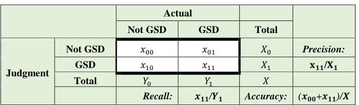
Table 5 General Confusion Matrix

Actual

Not GSD GSD Total

Judgment

Not GSD 𝑥𝑥₀₀ 𝑥𝑥₀₁ 𝑋𝑋₀ Precision:

GSD 𝑥𝑥₁₀ 𝑥𝑥₁₁ 𝑋𝑋₁ 𝐱𝐱_{𝟏𝟏𝟏𝟏}/𝐗𝐗_𝟏𝟏

Total 𝑌𝑌₀ 𝑌𝑌₁ 𝑋𝑋

Recall: 𝒙𝒙_{𝟏𝟏𝟏𝟏}/𝒀𝒀_𝟏𝟏 Accuracy: (𝒙𝒙_{𝟎𝟎𝟎𝟎}+𝒙𝒙_{𝟏𝟏𝟏𝟏})/𝑿𝑿

The common measures for assessing the appropriateness of the selection of

the best cut-off value 𝜌𝜌_{𝐺𝐺𝐺𝐺𝐺𝐺𝐿𝐿}are given by Recall = 𝑥𝑥₁₁/𝑌𝑌₁, Precision = 𝑥𝑥₁₁/𝑋𝑋₁ and Accuracy = (𝑥𝑥₀₀+𝑥𝑥₁₁)/𝑋𝑋. Recall describes the portion of actual GSDs that were judged to be a GSD, whereas Precision is the portion of judged GSDs that

were actually a GSD, and Accuracy represents the overall correctness of the

judgment.

It is clear that Recall decreases while Precision increases as 𝜌𝜌_{𝐺𝐺𝐺𝐺𝐺𝐺𝐿𝐿} increases. In order to balance the two conflicting measures, we consider the optimization

problem of maximizing Precision subject to Recall≥ 0.75 . This optimization problem is solved by varying 𝜌𝜌_{𝐺𝐺𝐺𝐺𝐺𝐺𝐿𝐿} with a stepwise of 0.01, yielding the best model with 𝜌𝜌∗_{𝐺𝐺𝐺𝐺𝐺𝐺𝐿𝐿} = 0.64 , Precision* = 0.81, Recall* = 0.76, and Accuracy* = 0.82. This optimal threshold 𝜌𝜌∗_{𝐺𝐺𝐺𝐺𝐺𝐺𝐿𝐿} corresponds tothe percentile points 𝑆𝑆₀∗= 3.591 million and𝑇𝑇₀∗= 2,870, representing the 80% and 70% levels of total sales and total number of purchase transactions in LD, respectively. The

resulting confusion matrix of the best model is shown in Table 6.

The estimated regression coefficients and other statistical measures of the

(15)

Table 6

Confusion Matrix With𝝆𝝆∗_{𝑮𝑮𝑮𝑮𝑮𝑮𝑮𝑮}= 𝟎𝟎.𝟔𝟔𝟔𝟔, 𝑺𝑺_𝟎𝟎∗ =𝟑𝟑,𝟖𝟖𝟖𝟖𝟔𝟔,𝟐𝟐𝟔𝟔𝟔𝟔 and 𝑻𝑻_𝟎𝟎∗ =𝟐𝟐,𝟗𝟗𝟔𝟔𝟗𝟗

Actual

¬ 𝑮𝑮𝑺𝑺𝑮𝑮 𝑮𝑮𝑺𝑺𝑮𝑮 Total

Judgment

¬ 𝑮𝑮𝑺𝑺𝑮𝑮 43 9 52 Precision

𝑮𝑮𝑺𝑺𝑮𝑮 7 29 36 80.6%

Total 50 38 88

Recall 76.3% Accuracy 81.8%

_{𝑮𝑮𝑺𝑺𝑮𝑮}: Good-Sales-Days, ¬ 𝑮𝑮𝑺𝑺𝑮𝑮: Not Good-Sales-Days

Table 7

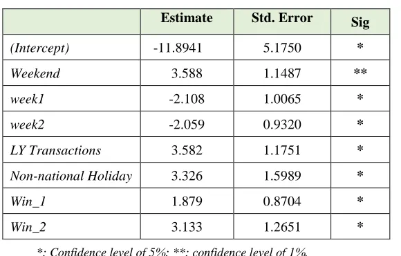
Estimated Coefficients of the Logistic Regression with𝝆𝝆∗_{𝑮𝑮𝑮𝑮𝑮𝑮𝑮𝑮}=𝟎𝟎.𝟔𝟔𝟔𝟔

𝑺𝑺𝟎𝟎∗ =𝟑𝟑,𝟖𝟖𝟖𝟖𝟔𝟔,𝟐𝟐𝟔𝟔𝟔𝟔 and 𝑻𝑻𝟎𝟎∗ =𝟐𝟐,𝟗𝟗𝟔𝟔𝟗𝟗

Estimate Std. Error _Sig

(Intercept) -11.8941 5.1750 *

Weekend 3.588 1.1487 **

week1 -2.108 1.0065 *

week2 -2.059 0.9320 *

LY Transactions 3.582 1.1751 *

Non-national Holiday 3.326 1.5989 *

Win_1 1.879 0.8704 *

Win_2 3.133 1.2651 *

*: Confidence level of 5%; **: confidence level of 1%.

Given the campaign day assignment, represented by 𝑎𝑎=

[𝑎𝑎(1),⋯,𝑎𝑎(𝑗𝑗),⋯,𝑎𝑎(𝑀𝑀)]∈{0,1}𝐶𝐶_{, where}

(16)

with ∑𝐶𝐶_𝑗𝑗=1𝑎𝑎(𝑗𝑗)≤ 𝑁𝑁,𝑎𝑎nd the explanatory variables for day𝑗𝑗 in Table 7, the logistic regression model can be used to define 𝐼𝐼̂_{𝐺𝐺𝐺𝐺𝐺𝐺𝐿𝐿}(𝑗𝑗) as:

𝐼𝐼̂𝐺𝐺𝐺𝐺𝐺𝐺𝐿𝐿∗ (𝑗𝑗) =�1 , 𝑖𝑖𝑖𝑖𝜌𝜌𝐺𝐺𝐺𝐺𝐺𝐺𝐿𝐿(𝑗𝑗)≥ 𝜌𝜌 ∗

𝐺𝐺𝐺𝐺𝐺𝐺𝐿𝐿

0 , 𝑒𝑒𝑒𝑒𝑠𝑠𝑒𝑒 . (3.7)

This in turn enables one to estimate the expected total sales per day in a future

period, which is a vital step toward deciding the optimal campaign day assignment

𝑎𝑎∗_{and the optimal budget size}_𝐵𝐵∗_{so as to maximize the expected total profit, as} we discuss next.

3.3. Step III: Estimating Expected Total Sales per Day in 𝑮𝑮_{𝑻𝑻𝑮𝑮}

We now turn to the issue of how to estimate the expected total sales of day𝑗𝑗,

𝑗𝑗 ∈ 𝐷𝐷𝑇𝑇𝐿𝐿 in the future winter period. For this purpose, we compute the average total sales, denoted by 𝑠𝑠̂₍_𝑚𝑚_,_𝑛𝑛₎, over the learning period 𝑖𝑖 ∈ 𝐷𝐷_{𝐿𝐿𝐿𝐿} with 𝑐𝑐=

𝐼𝐼𝐶𝐶𝐶𝐶𝐶𝐶𝐶𝐶(𝑖𝑖) and 𝑊𝑊=𝐼𝐼𝐺𝐺𝐺𝐺𝐺𝐺𝐿𝐿:𝑆𝑆0∗𝑇𝑇0∗(𝑖𝑖),𝑐𝑐,𝑊𝑊 ∈{0,1} as shown in Table 8, resulting in

four values of the average total sales obtained from LD; that is, 𝑠𝑠̂₍₀_,₀₎= ¥ 3.65 m,

𝑠𝑠̂(0,1)= ¥ 4.68 m, 𝑠𝑠̂(1,0)= ¥ 3.89 m, 𝑠𝑠̂(1,1)= ¥ 4.82 m (m: million).

Table 8

Average Total Sales Matrix 𝒔𝒔�₍_𝒎𝒎_,_𝑾𝑾₎ in ¥ Million Based on LD

𝑮𝑮𝑵𝑵𝑵𝑵𝑾𝑾 − 𝑺𝑺𝑾𝑾𝑵𝑵𝑾𝑾𝒔𝒔 − 𝑮𝑮𝑾𝑾𝑾𝑾

0 1

𝑪𝑪𝑾𝑾𝒎𝒎𝑪𝑪𝑾𝑾𝒊𝒊𝑪𝑪𝑾𝑾 𝑮𝑮𝑾𝑾𝑾𝑾

0 𝑠𝑠̂(0,0) 𝑠𝑠̂(0,1)

1 𝑠𝑠̂(1,0) 𝑠𝑠̂(1,1)

The expected total sales per day in 𝐷𝐷_{𝑇𝑇𝐿𝐿} should be estimated by taking into consideration the effect of the enhanced campaign budget. More specifically, let

𝐵𝐵0 be the standard budget and define the enhanced campaign budget per day

(17)

Two main settings are considered. First, if day 𝑗𝑗 ∈ 𝐷𝐷_{𝑇𝑇𝐿𝐿} in the future winter period under consideration is not chosen for the sales campaign (that is, if𝑎𝑎(𝑗𝑗) = 0), the campaign budget will not have an effect on the expected total sales of day𝑗𝑗. Second, if day 𝑗𝑗 is chosen for the sales campaign (that is, if𝑎𝑎(𝑗𝑗) = 1), it is natural to assume that the expected total sales would increase as ∆_𝐵𝐵 increases with the effect of diminishing return. This effect may depend on whether or not day 𝑗𝑗 of

𝐷𝐷𝐿𝐿𝐿𝐿 was under the sales campaign. The effect of the former case is represented by𝑐𝑐_{𝐶𝐶𝐶𝐶𝐶𝐶𝐶𝐶→𝐶𝐶𝐶𝐶𝐶𝐶𝐶𝐶}(∆_𝐵𝐵) and that of the latter case by 𝑐𝑐_¬_{𝐶𝐶𝐶𝐶𝐶𝐶𝐶𝐶→𝐶𝐶𝐶𝐶𝐶𝐶𝐶𝐶}(∆_𝐵𝐵), where both functions are strictly increasing and concave in ∆_𝐵𝐵 with 𝑐𝑐_{𝐶𝐶𝐶𝐶𝐶𝐶𝐶𝐶→𝐶𝐶𝐶𝐶𝐶𝐶𝐶𝐶}(0) =

𝑐𝑐¬𝐶𝐶𝐶𝐶𝐶𝐶𝐶𝐶→𝐶𝐶𝐶𝐶𝐶𝐶𝐶𝐶(0) = 1.

More specifically, let 𝑟𝑟̂₍_𝑚𝑚_,_𝑛𝑛₎_{→�𝑚𝑚}_:

∆𝐵𝐵,𝑛𝑛:∆𝐵𝐵�(𝑗𝑗) be the expected total sales of

day 𝑗𝑗 in 𝐷𝐷_{𝑇𝑇𝐿𝐿} estimated when day 𝑗𝑗 in 𝐷𝐷_{𝐿𝐿𝐿𝐿} had 𝑐𝑐=𝐼𝐼_{𝐶𝐶𝐶𝐶𝐶𝐶𝐶𝐶}(𝑗𝑗) and 𝑊𝑊=

𝐼𝐼𝐺𝐺𝐺𝐺𝐺𝐺𝐿𝐿: 𝑆𝑆0𝑇𝑇0(𝑗𝑗), and day 𝑗𝑗 in 𝐷𝐷𝑇𝑇𝐿𝐿 has 𝑐𝑐:∆𝐵𝐵=𝑎𝑎(𝑗𝑗), and 𝐼𝐼̂𝐺𝐺𝐺𝐺𝐺𝐺𝐿𝐿∗ (𝑗𝑗). One then has: 𝑟𝑟̂(0,𝑛𝑛)→(0,𝑛𝑛:_∆𝐵𝐵)(𝑗𝑗) = 𝑠𝑠̂(0,𝑛𝑛), 𝑊𝑊,𝑊𝑊:∆𝐵𝐵 ∈{0,1},

𝑟𝑟̂(0,𝑛𝑛)→(1,𝑛𝑛:_∆𝐵𝐵)(𝑗𝑗) = 𝑠𝑠̂(0,𝑛𝑛) ×𝑐𝑐¬𝐶𝐶𝐶𝐶𝐶𝐶𝐶𝐶→𝐶𝐶𝐶𝐶𝐶𝐶𝐶𝐶(∆𝐵𝐵) , 𝑊𝑊, ,𝑊𝑊:∆𝐵𝐵 ∈{0,1}, ∆𝐵𝐵

> 0 (3.8)

𝑟𝑟̂(1,𝑛𝑛)→(1,𝑛𝑛:_∆𝐵𝐵)(𝑗𝑗) = 𝑠𝑠̂(1,𝑛𝑛) ×𝑐𝑐𝐶𝐶𝐶𝐶𝐶𝐶𝐶𝐶→𝐶𝐶𝐶𝐶𝐶𝐶𝐶𝐶(∆𝐵𝐵), 𝑊𝑊, ,𝑊𝑊:∆𝐵𝐵∈{0,1}, ∆𝐵𝐵> 0

Accordingly, the aggregated total expected sales, denoted by𝑅𝑅��𝑎𝑎, ∆_𝐵𝐵�, can be obtained as

𝑅𝑅��𝑎𝑎,∆𝐵𝐵�=

� � 𝑟𝑟̂₍_𝑚𝑚_,_𝑛𝑛₎_{→�𝑚𝑚}_:_∆𝐵𝐵_,_𝑛𝑛_:_∆𝐵𝐵_�(𝑗𝑗) 𝛿𝛿{𝐼𝐼𝐶𝐶𝐶𝐶𝐶𝐶𝐶𝐶(𝑖𝑖)=𝑚𝑚}𝛿𝛿{𝐼𝐼𝐺𝐺𝐺𝐺𝐺𝐺𝐿𝐿: 𝑆𝑆0𝑇𝑇0(𝑖𝑖)=𝑛𝑛}𝛿𝛿{𝑑𝑑(𝑗𝑗)=𝑚𝑚:∆𝐵𝐵}

𝑚𝑚,𝑛𝑛∈{0,1}

𝛿𝛿{𝐼𝐼̂𝐺𝐺𝐺𝐺𝐺𝐺𝐿𝐿∗ (𝑗𝑗)=𝑛𝑛:_∆𝐵𝐵},

𝐶𝐶

𝑗𝑗=1

(3.9),

(18)

Before moving to the last step, we construct the two functions

𝑐𝑐𝐶𝐶𝐶𝐶𝐶𝐶𝐶𝐶→𝐶𝐶𝐶𝐶𝐶𝐶𝐶𝐶(∆𝐵𝐵) and 𝑐𝑐¬𝐶𝐶𝐶𝐶𝐶𝐶𝐶𝐶→𝐶𝐶𝐶𝐶𝐶𝐶𝐶𝐶(∆𝐵𝐵) explicitly. For this purpose, we use a generic function 𝑐𝑐(∆_𝐵𝐵) of the form

𝑐𝑐(∆𝐵𝐵) = 1 +_{1 +}𝑎𝑎 _𝑏𝑏∙ ∆_∙𝐵𝐵_∆

𝐵𝐵 . (3.10)

By differentiating 𝑐𝑐(∆_𝐵𝐵) twice with respect to∆_𝐵𝐵 , one sees that

𝑎𝑎

𝑎𝑎𝑥𝑥 𝑐𝑐(∆𝐵𝐵) =

𝑎𝑎(1 +𝑏𝑏 ∙ ∆𝐵𝐵)− 𝑎𝑎𝑏𝑏 ∙ ∆𝐵𝐵 (1 +𝑏𝑏 ∙ ∆𝐵𝐵)2 =

𝑎𝑎

(1 +𝑏𝑏 ∙ ∆𝐵𝐵)2 > 0 (3.11) and

𝑎𝑎2

𝑎𝑎𝑥𝑥2 𝑐𝑐(∆𝐵𝐵) = − 2𝑏𝑏 _{(1 +}_𝑏𝑏𝑎𝑎 _{∙ ∆}

𝐵𝐵)3 < 0 ,𝑤𝑤ℎ𝑒𝑒𝑊𝑊 ∆𝐵𝐵> 0 (3.12) We note that 𝑐𝑐(∆_𝐵𝐵) is strictly increasing and concave in∆_𝐵𝐵. Furthermore, it can be seen that

𝑒𝑒𝑖𝑖𝑐𝑐

∆𝐵𝐵→∞𝑐𝑐(∆𝐵𝐵) = 1 + 𝑎𝑎

𝑏𝑏 (3.13)

The functions g_CAMP→CAMP(∆_B) and g¬_CAMP→CAMP(∆_B) can then be

constructed by setting different values of a and b; that is,

𝑐𝑐𝐶𝐶𝐶𝐶𝐶𝐶𝐶𝐶→𝐶𝐶𝐶𝐶𝐶𝐶𝐶𝐶(∆𝐵𝐵) = 1 +_{1 +}𝑎𝑎𝑠𝑠_𝑏𝑏∙ ∆𝐵𝐵 𝑠𝑠∙ ∆𝐵𝐵 , 𝑐𝑐¬𝐶𝐶𝐶𝐶𝐶𝐶𝐶𝐶→𝐶𝐶𝐶𝐶𝐶𝐶𝐶𝐶(∆𝐵𝐵) = 1 +_{1 +}𝑎𝑎¬_𝑏𝑏𝑠𝑠∙ ∆𝐵𝐵

¬𝑠𝑠 ∙ ∆𝐵𝐵 . (3.14)

3.4. Step IV: Formulating the Optimization Problem for Maximizing Expected Profit

The optimization problem of expected profit, denoted by 𝑃𝑃��𝑎𝑎,∆_𝐵𝐵� , can be readily formulated as follows:

𝑃𝑃��𝑎𝑎∗_,_∆ 𝐵𝐵

∗_�_{= max}

𝑑𝑑_∆𝐵𝐵, ∆𝐵𝐵 �𝑅𝑅��𝑎𝑎, ∆𝐵𝐵� −(𝐵𝐵0+∆𝐵𝐵) ×� 𝑎𝑎(𝑗𝑗)

𝐶𝐶

𝑗𝑗=1

(19)

subject to the campaign budget increase being 0 <𝐵𝐵₀+∆_𝐵𝐵≤ 𝐵𝐵_{𝐶𝐶𝑀𝑀𝑀𝑀} , and∑𝐶𝐶_𝑗𝑗=1𝑎𝑎_∆_𝐵𝐵(𝑗𝑗)≤ 𝑁𝑁, where 𝑁𝑁 is the actual number of sales campaign days organized over the learning data of Winter 2010.

4. NUMERICAL RESULTS FOR THE WINTER PERIOD

In order to define 𝑐𝑐_{𝐶𝐶𝐶𝐶𝐶𝐶𝐶𝐶→𝐶𝐶𝐶𝐶𝐶𝐶𝐶𝐶}(∆_𝐵𝐵) and 𝑐𝑐_¬_{𝐶𝐶𝐶𝐶𝐶𝐶𝐶𝐶→𝐶𝐶𝐶𝐶𝐶𝐶𝐶𝐶}(∆_𝐵𝐵) appropriately based on (3.14), we investigate the effect of varying two parameters 𝑎𝑎 and𝑏𝑏 on the value of𝑐𝑐(∆_𝐵𝐵) under two constraints, 𝑎𝑎 >𝑏𝑏 or 𝑎𝑎<𝑏𝑏, with 0 <∆_𝐵𝐵≤ 2 𝐵𝐵0. Figure 3(A) shows the case when 𝑎𝑎 is kept constant at 𝑎𝑎=5 with varying parameter 𝑏𝑏 ∈ 𝐵𝐵= { 1 , ⋯ , 10 }, and Figure 3(B) shows the case when 𝑏𝑏 is kept constant at 𝑏𝑏=5 with varying parameter𝑎𝑎 ∈ 𝐴𝐴= { 1 ,⋯ , 10}. Similar graphs are observed when 𝑎𝑎 and 𝑏𝑏 are fixed at different levels.

To determine (𝑎𝑎_𝑠𝑠 ,𝑏𝑏_𝑠𝑠) and (𝑎𝑎_¬_𝑠𝑠 ,𝑏𝑏_¬_𝑠𝑠),we first compute all possible combinations of (𝑎𝑎_𝑠𝑠 ,𝑏𝑏_𝑠𝑠), (𝑎𝑎_¬_𝑠𝑠 ,𝑏𝑏_¬_𝑠𝑠) ∈{1,⋯, 10} × {1,⋯, 10} satisfying

𝑎𝑎𝑠𝑠 <𝑏𝑏𝑠𝑠and 𝑎𝑎¬𝑠𝑠<𝑏𝑏¬𝑠𝑠. Then, each of the resulting maximum total profits is compared against the actual total sales, minus the corresponding campaign cost.

The appropriate choices of (𝑎𝑎_𝑠𝑠 ,𝑏𝑏_𝑠𝑠) and (𝑎𝑎_¬_𝑠𝑠 ,𝑏𝑏_¬_𝑠𝑠) are determined by selecting the ones that achieve the minimum absolute difference, resulting in (𝑎𝑎_𝑠𝑠,𝑏𝑏_𝑠𝑠) = (9, 10) and (𝑎𝑎_¬_𝑠𝑠,𝑏𝑏_¬_𝑠𝑠) = (6, 7). These parameter values are rather insensitive to the final maximum expected profit, as shown in equation (4.1). Furthermore, the

sensitivity index SI is computed where 𝑃𝑃��𝑎𝑎∗,∆_𝐵𝐵∗�

𝐶𝐶𝐶𝐶𝑀𝑀 is the maximum possible value of 𝑃𝑃��𝑎𝑎∗,∆_𝐵𝐵∗� in (3.15) over all combinations of (𝑎𝑎_𝑠𝑠 ,𝑏𝑏_𝑠𝑠), (𝑎𝑎_¬_𝑠𝑠 ,𝑏𝑏_¬_𝑠𝑠) ∈ {1,⋯, 10} × {1,⋯, 10} satisfying 𝑎𝑎_𝑠𝑠<𝑏𝑏_𝑠𝑠and 𝑎𝑎_¬_𝑠𝑠 <𝑏𝑏_¬_𝑠𝑠 and 𝑃𝑃��𝑎𝑎∗,∆_𝐵𝐵∗�

𝐶𝐶𝐼𝐼𝑁𝑁 is defined similarly for the minimum possible value, yielding:

𝑆𝑆𝐼𝐼= 𝑃𝑃��𝑎𝑎 ∗_,_∆

𝐵𝐵 ∗_�

𝐶𝐶𝐶𝐶𝑀𝑀− 𝑃𝑃��𝑎𝑎∗,∆𝐵𝐵∗�𝐶𝐶𝐼𝐼𝑁𝑁

𝑃𝑃��𝑎𝑎∗_,_∆ 𝐵𝐵 ∗_�

𝐶𝐶𝐶𝐶𝑀𝑀

= 156.14 _156.14− 146.95= 0.059 . (4.1) The two functions 𝑐𝑐_{𝐶𝐶𝐶𝐶𝐶𝐶𝐶𝐶→𝐶𝐶𝐶𝐶𝐶𝐶𝐶𝐶}(∆_𝐵𝐵) with (𝑎𝑎_𝑠𝑠,𝑏𝑏_𝑠𝑠) = (9, 10) and

(20)

F

ig

u

re

3(

A

) an

d

3(

B

).

B

eh

avi

or

o

f

𝑪𝑪

(

∆𝑩𝑩

)

f

o

r

𝟎𝟎

<

∆𝑩𝑩

≤

𝟐𝟐𝑩𝑩

(21)

F ig u re 4 (A ) a n d 4 (B ). 𝑪𝑪𝑪𝑪𝑪𝑪𝑪𝑪 𝑪𝑪 → 𝑪𝑪𝑪𝑪 𝑪𝑪 𝑪𝑪 ( ∆𝑩𝑩 ) a nd 𝑪𝑪¬𝑪𝑪𝑪𝑪𝑪𝑪 𝑪𝑪 → 𝑪𝑪𝑪𝑪𝑪𝑪 𝑪𝑪 (∆𝑩𝑩 ) w

(22)

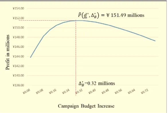
With the standard campaign budget given by the shopping center to be 𝐵𝐵₀= ¥ 0.4 million per day, the expected total profit 𝑃𝑃��𝑎𝑎∗,∆_𝐵𝐵�maximized over𝑎𝑎 given

∆𝐵𝐵 per day is exhibited as a function of∆𝐵𝐵, yielding the final optimal expected profit of 𝑃𝑃��𝑎𝑎∗,∆_𝐵𝐵∗�= ¥ 151.49 million, with the optimal budget increase of∆_𝐵𝐵∗= ¥ 0.32 million (Figure 5).

Figure 5. Expected Total Profit 𝑪𝑪��𝑾𝑾∗(∆_𝑩𝑩),∆_𝑩𝑩�Maximized over𝑾𝑾 Given ∆_𝑩𝑩

The difference between the actual total sales minus the corresponding sales

campaign cost obtained from the real data and 𝑃𝑃��𝑎𝑎∗,∆_𝐵𝐵∗�= ¥ 151.49 million is compared with the actual profit 𝑃𝑃�𝐼𝐼_{𝐶𝐶𝐶𝐶𝐶𝐶𝐶𝐶}�= ¥ 129.7 million, yielding a 16.8% increase in expected profit by reallocating 23 sales campaign days over the winter

period with an optimal sales campaign budget per day of 𝐵𝐵∗= ¥ 0.72 million

(23)

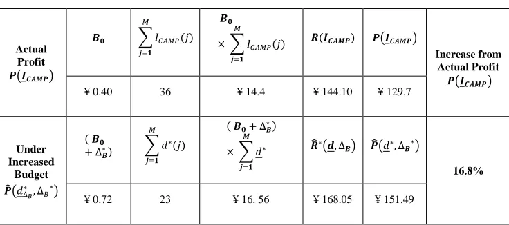
Table 9

Actual and Optimal Profits under Increased Budget for Winter 2011 (TD)

Actual Profit 𝑪𝑪�𝑰𝑰𝑪𝑪𝑪𝑪𝑪𝑪𝑪𝑪� 𝑩𝑩𝟎𝟎 � 𝐼𝐼𝐶𝐶𝐶𝐶𝐶𝐶𝐶𝐶(𝑗𝑗) 𝑪𝑪 𝒋𝒋=𝟏𝟏 𝑩𝑩𝟎𝟎 × � 𝐼𝐼𝐶𝐶𝐶𝐶𝐶𝐶𝐶𝐶(𝑗𝑗) 𝑪𝑪 𝒋𝒋=𝟏𝟏 𝑹𝑹(𝑰𝑰𝑪𝑪𝑪𝑪𝑪𝑪𝑪𝑪) 𝑪𝑪�𝑰𝑰𝑪𝑪𝑪𝑪𝑪𝑪𝑪𝑪� Increase from Actual Profit 𝑪𝑪�𝑰𝑰𝑪𝑪𝑪𝑪𝑪𝑪𝑪𝑪�

¥ 0.40 36 ¥ 14.4 ¥ 144.10 ¥ 129.7

Under Increased Budget 𝑪𝑪��𝑎𝑎∆∗𝐵𝐵,∆𝐵𝐵∗� ( 𝑩𝑩𝟎𝟎 +∆𝑩𝑩∗) � 𝑎𝑎 ∗₍_𝑗𝑗₎ 𝑪𝑪 𝒋𝒋=𝟏𝟏 ( 𝑩𝑩𝟎𝟎+∆𝑩𝑩∗) × � 𝑎𝑎∗ 𝑪𝑪 𝒋𝒋=𝟏𝟏 𝑹𝑹�∗_�𝑾𝑾_,_∆ 𝑩𝑩� 𝑪𝑪��𝑎𝑎∗,∆𝑩𝑩∗� 16.8%

¥ 0.72 23 ¥ 16. 56 ¥ 168.05 ¥ 151.49

Table 10 presents the number of sales campaign days (SCDs) in actual practice

and the optimal solution. The optimal solution𝑃𝑃��𝑎𝑎∗,∆_𝐵𝐵∗� is achieved by allocating 7 and 2 days in December and January, respectively, and 14 days in February,

compared with 0 in actual practice.

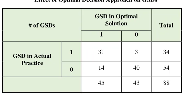
Table 11 indicates how GSDs were optimally allocated compared with actual

practice. One observes that 42 days were judged as GSDs under the optimal

decision, compared with 34 GSDs in actual practice, which amounts to a 23.5%

(8/34) increase in GSDs in the optimal decision.

Table 10

Number of SCDs Allocated in Actual Practice and Under Optimal Solution, Winter 2011

Month Actual Number of Campaign Days

Optimal Number of Campaign Days

December 28 7

January 8 2

February 0 14

(24)

Table 11

Effect of Optimal Decision Approach on GSDs

# of GSDs

GSD in Optimal

Solution _Total

1 0

GSD in Actual Practice

1 31 3 34

0 14 40 54

45 43 88

Table 12 presents further details on how the above improvement by the

optimal decision approach was achieved, where GSD versus ￢GSD transitions

are classified according to sales campaign days only in actual practice, those in

common, and those only by the optimal decision approach.

In actual practice, 15+1=16 were assigned as GSDs [that is, 44% (16/36)] and

55.5% (20/36) were assigned as￢GSD. In contrast, the optimal decision

approach allocated only 8+1=9 days (or 39%) to GSDs in actual practice and 11+3

= 14 days (or 60%) to￢GSD. This result supports the original observation that the

effect of a sales campaign on enhancing the total sales of ￢GSD may exceed that

of strengthening the total sales of GSD further. This result is also consistent with

that reported in Sharkasi, Yoshi, and Sumita (2015).

(25)

(26)

5. CONCLUSION AND DISCUSSION

An extensive literature exists concerning shopping centers and related sales

optimization, where different approaches are taken; e.g., how to find the optimal

allocation of SCs among available alternatives and how to determine the

configuration of space and design so as to achieve either cost-performance

efficiency or profit generation. To the best of our knowledge, however, the

problem of optimally allocating campaign days over a certain period (e.g., the

winter season) has not been addressed in the literature. This paper is an extension

of Sharkasi et al. (2015). It aimed to investigate the effect of flexible allocation of

sales campaign days on expected total profit by incorporating the campaign budget

per day as part of the optimization problem. For this purpose, the impact of budget

increments on revenue was incorporated by defining a concave function to exhibit

the effect of diminishing returns.

Through numerical examples involving actual data from a shopping center in

Tokyo, the proposed model showed that expected profit can be maximized by

optimal allocation of sales campaign days and campaign budget, achieving a

16.8% increase in expected profit with fewer sales campaign days by improving

the sales campaign budget per day by 80%. The management of a shopping center

can better serve its tenants by using this systematic approach to optimize the

assignment and budgeting of sales campaign days.

With respect to limitations of the current study, the optimized profit in this

study was gross profit and not net profit or net earnings because of limited data

access from the shopping center.

It should be noted that this optimization problem took into consideration a

constraint of a minimum number of days organized during the Christmas season

in order to meet the realistic goals of an SC. It should also be noted that numerical

results obtained from applying this systematic approach to the fall period yielded

(27)

it could still be considered to solve the problem proposed in this paper because the

standing managerial practice of SCs to schedule sales campaign days in the current

year with reference to the previous year’s schedule remains unchanged.

A possibility for future research could be optimizing net profit by further

taking into consideration the possible impact of the proposed flexible assignment

of sales campaign days on the marketing cost structure. Two assumptions could be

laid forward. First, the flexible allocation of sales campaign days could exhaust the

cost structure because of increased spending on advertising to reach out to

prospects to inform them of possible fragmented assignment of sales campaign

days. The second assumption could be quite contrasting. With the current pressure

on brick-and-mortar SCs to reduce costs under intensifying competition from

contemporary online and mobile shopping platforms, SCs may be able to leverage

the power of smartphones to connect with prospects intelligently through GPS

capability. This way, the SC could generate massive customized alerts with meager

additional costs in the promise of maximizing revenue through optimal allocation

of sales campaign days. Based on the managerial style of implementing the

proposed approach of flexible allocation of sales campaign days, the optimization

problem of net profit could be structured and solved accordingly.

ACKNOWLEDGEMENT

The authors would like to thank the anonymous reviewers for their kind suggestions that lead to further improve the paper.

REFERENCES

Ahmadi-Javid, A.; Amiri, E.; and Meskar, M. (2018). A profit-maximization location-routing-pricing problem: A branch-and-price algorithm, European Journal of Operational Research (in press; available online 25 February 2018). DOI:

(28)

International Journal of Business and Information Balaghar, A.; Majidazar M.; and Niromand M. (2012). Evaluation of effectiveness of sales promotional tools on sales volume – Case study: Iran tractor manufacturing complex (IT MC), Middle-East Journal of Scientific Research 11 (4), 470- 480. Bhattacharjee, S., and Ramesh, R. (2000). A multi-period profit maximizing model for

retail supply chain management: An integration of demand and supply-side

mechanisms, European Journal of Operational Research 122(3), 584-601. DOI: 10.1016/s0377-2217(99)00097-1

Burns, D.J., and Warren, H.B. (1995, 12). Need for uniqueness: Shopping mall preference and choice activity, International Journal of Retail & Distribution Management 23(12), 4-12. DOI: 10.1108/09590559510103954

Chapados, N.; Joliveau, M.; L’Ecuyer, P.; and Rousseau, L. (2014). Retail store scheduling for profit, European Journal of Operational Research 239(3), 609-624. DOI: 10.1016/j.ejor.2014.05.033

Christaller, W., and Baskin, C.W. (1966). Central Places in Southern Germany. Englewood Cliffs, NJ: Prentice-Hall.

Eckert, A.; He, Z.; and West, D.S. (2015). An empirical analysis of tenant location patterns near department stores in planned regional shopping centers, Journal of Retailing and Consumer Services 22, 61-70.

DOI: 10.1016/j.jretconser.2014.09.007

Eppli, M.J., and Benjamin, J.D. (1994). The evolution of shopping center research: A review and analysis, Journal of Real Estate Research 9(1), 5-32.

(29)

Groover, M.P. (1987). Automation, Production Systems and Computer-Integrated

Manufacturing, Upper Saddle River, New Jersey: Prentice-Hall Publishers.

DOI: https://doi.org/10.1108/aa.2002.22.3.298.2

Heuvel, W.V., and Wagelmans, A P. (2017). A note on ‘A multi-period profit maximizing model for retail supply chain management,’ European Journal of Operational Research 260(2), 625-630. DOI: 10.1016/j.ejor.2017.01.014

Hübner, A.; Kuhn, H.; and Kühn, S. (2016). An efficient algorithm for capacitated assortment planning with stochastic demand and substitution, European Journal of Operational Research 250(2), 505-520. DOI: 10.1016/j.ejor.2015.11.007

Irion, J.; Lu, J.; Al-Khayyal, F.; and Tsao, Y. (2012). A piecewise linearization framework for retail shelf space management models, European Journal of Operational Research 222(1), 122-136. DOI: 10.1016/j.ejor.2012.04.021

Jeffery, M. (2010). Data-Driven Marketing: The 15 Metrics Everyone in Marketing Should Know, New York: John Wiley Publishers. DOI: 10.1002/9781119198666

Jones, E. (1997). An analysis of consumer food shopping behavior using supermarket scanner data: Differences by income and location, American Journal of Agricultural Economics 79(5), 1437. DOI: 10.2307/1244358

Kabak, Ö.; Ülengin, F.; Aktaş, E.; Önsel, Ş.; and Topcu, Y.I. (2008). Efficient shift scheduling in the retail sector through two-stage optimization, European Journal of Operational Research 184(1), 76-90. DOI: 10.1016/j.ejor.2006.10.039

Katsifou, A.; Seifert, R.W.; and Tancrez, J. (2014). Joint product assortment, inventory and price optimization to attract loyal and non-loyal customers, Omega 46, 36-50. DOI: 10.1016/j.omega.2014.02.002

Kumar, V.; Shah, D.; and Venkatesan, R. (2006). Managing retailer profitability—one customer at a time! Journal of Retailing 82(4), 277-294.

(30)

International Journal of Business and Information Lehew, M.L., and Fairhurst, A.E. (2000). U.S. shopping mall attributes: An exploratory investigation of their relationship to retail productivity, International Journal of Retail & Distribution Management 28(6), 261-279.

DOI: 10.1108/09590550010328535

Muhlebach, R.F., and Alexander, A.A. (2019). Shopping Center Management and Leasing, Institute of Real Estate Management.

Murray, C.C.; Talukdar, D.; and Gosavi, A. (2010). Joint optimization of product price, display orientation and shelf-space allocation in retail category management, Journal of Retailing 86(2), 125-136. DOI: 10.1016/j.jretai.2010.02.008

Sharkasi,N.; Sumita, U.; and Yoshii, J. (2014). Development of enhanced marketing flexibility by optimally allocating sales campaign days for maximizing total expected sales, Global Journal of Flexible Systems Management 16(1), 87-95.

DOI: 10.1007/s40171-014-0082-9

Parsons, A.G. (2003). Assessing the effectiveness of shopping mall promotions: Customer analysis, International Journal of Retail and Distribution Management 31(2), 74-79. DOI: 10.1108/09590550310461976

Rambha, T.; Boyles, S.D.; Unnikrishnan, A.; and Stone, P. (2018). Marginal cost pricing for system optimal traffic assignment with recourse under supply-side uncertainty, Transportation Research Part B: Methodological 110, 104-121. DOI: 10.1016/j.trb.2018.02.008

Shim, S., and Eastlick, M.A. (1998). The hierarchical influence of personal values on mall shopping attitude and behavior, Journal of Retailing 74(1), 139-160.

DOI: 10.1016/s0022-4359(99)80091-8

(31)

Wakefield, K.L., and Baker, J. (1998). Excitement at the mall: Determinants and effects on shopping response, Journal of Retailing 74(4), 515-539.

DOI: 10.1016/s0022-4359(99)80106-7

Wang, X., and Li, D. (2012). A dynamic product quality evaluation-based pricing model for perishable food supply chains, Omega 40(6), 906-917.

DOI: 10.1016/j.omega.2012.02.001

Wang, Y., and Li, L. (2017). Manufacturing profit maximization under time-varying electricity and labor pricing, Computers and Industrial Engineering 104, 23-34. DOI: 10.1016/j.cie.2016.12.011

Weber, J. (1969). Evidence for discovery of gravitational radiation, Physical Review Letters 22(24), 1320-1324. DOI: 10.1103/physrevlett.22.1320

Yada, K.; Motoda, H.; Washio, T.; & Miyawaki, A. (2004). Consumer behavior analysis by graph mining technique, Lecture Notes in Computer Science Knowledge-Based Intelligent Information and Engineering Systems, 800-806.

DOI:10.1007/978-3-540-30133-2_105

Yu, B., Yang, Z., & Cheng, C. (2007). Optimizing the distribution of shopping centers with parallel genetic algorithm. Engineering Applications of Artificial Intelligence, 20(2), 215-223. DOI: 10.1016/j.engappai.2006.06.015

ABOUT THE AUTHORS

(32)

International Journal of Business and Information technology and telecommunications companies both in Japan and the U.S., as well as government organizations in Japan and other countries.

Ushio Sumita is Professor Emeritus at the University of Tsukuba, Japan. He currently teaches in the Graduate School of Business Administration, Keio University, Japan, and at the Graduate School of International Management at the International University of Japan. He also serves as a technical advisor for the Information Science Department, Information Systems Division, LIXIL Corporation, and for Matsuda Electronic Engineering Corporation. He received his first Ph.D. in 1981 from the University of Rochester, Rochester, New York, U.S.A., and his second Ph.D. in 1987 from Tokyo Institute of Technology, Japan. He has a broad range of research interests and has published more than 170 papers in leading archive journals in such areas as information technology, big data analytics, artificial intelligence, financial engineering, marketing, operations management, operations research, and organization theory. He has also conducted rigorous mathematical analyses in the areas of applied probability, stochastic processes, and queuing theory. Ushio has been involved in various consulting activities in numerous areas including IoT, big data analytics, new product development, logistics, value chain management, information technology, e-business, digital marketing, financial engineering, human resources management, and business process management.