Performance Evaluation of Spatial Modulation and QOSTBC for MIMO Systems

Performance Evaluation of Spatial Modulation and

QOSTBC for MIMO Systems

†

K.O.O. Anoh1, R.A. Abd-Alhameed1,*, G.N. Okorafor2, J.M. Noras1, J. Rodriguez1,3 and S.M.R. Jones1

1_{School of Electrical Engineering and Computer Science, University of Bradford, UK}

2_{Dept. of Electrical and Electronics Engineering, Federal University of Technology, Owerri-Nigeria} 3_{Instituto de Telecomunicações - Aveiro Campus, Universitário de, Santiago, Aveiro, Portugal}

Abstract

Multiple-input multiple-output (MIMO) systems require simplified architectures that can maximize design parameters without sacrificing system performance. Such architectures may be used in a transmitter or a receiver. The most recent example with possible low cost architecture in the transmitter is spatial modulation (SM). In this study, we evaluate the SM and quasi-orthogonal space time block codes (QOSTBC) schemes for MIMO systems over a Rayleigh fading channel. QOSTBC enables STBC to be used in a four antenna design, for example. Standard QO-STBC techniques are limited in performance due to self-interference terms; here a QOSTBC scheme that eliminates these terms in its decoding matrix is explored. In addition, while most QOSTBC studies mainly explore performance improvements with different code structures, here we have implemented receiver diversity using maximal ratio combining (MRC). Results show that QOSTBC delivers better performance, at spectral efficiency comparable with SM.

1. Introduction

Since the demand for ever higher data rates is a major driver in research on telecommunications services for mobile devices, modern (and future) telecommunication standards are being proposed based on multiple-input multiple-output (MIMO) antenna configurations. In long-term evolution (LTE) and LTE-Advanced (LTE-A) for example, data rates on the Gigabit scale are being sought [1]. The MIMO scheme exploits the probability that no two channel paths will have equally bad impairments, thus increasing the number of transmitting and/or receiver elements can improve the probability of correctly receiving transmitted information over a fading channel. For instance, if p is the probability that the instantaneous signal-to-noise ratio (SNR) falls below a critical value on each antenna branch

(usually called the outage probability [2]), then _p(NR)_{is the}

probability that the instantaneous SNR is below the same critical value on all NR-receiver branches for independently faded channels [3]. Since mobile receivers are generally compact, diversity techniques are best utilised in the transmitter.

MIMO schemes increase both transmitter and receiver diversity beyond one antenna. Many different transmitter diversity techniques have been studied by researchers [4]. Maximal ratio combing (MRC) is an optimum combining method for flat fading channels with additive white Gaussian noise (AWGN) [4] and is applied in the receiver.

Examples of popular transmitter diversity techniques include spatial multiplexing and space-time block coding (STBC). Most recently, the spatial modulation (SM) technique [5, 6] has been introduced. In SM, multiple antenna systems are designed with only one radio frequency (RF) chain in the transmitter. This technique is explored in this study and will be compared with QOSTBC alongside STBC. The standard QOSTBC scheme is limited by non-zero off-diagonal terms in its detection matrix. Here, a QOSTBC scheme that does not have this limitation is used. In this paper, this will be referred to as interference-free QOSTBC.

Spatial modulation (SM) is an attractive multi-antenna transceiver technique for MIMO system deployment. It improves spectral efficiency and has no inter-channel interference (ICI) at the receiver, provided the pulse shaping period does not overlap amongst antennas [7]. SM reduces transmitter complexity and cost since only one transmitting antenna is activated during a transmission period, thus reducing the number of RF-chains to one. When SM was introduced, it was compared with STBC which uses up to 4-receiver antennas [8]. STBC improves power efficiency by maximizing spatial diversity, and improves capacity from diversity gain, which reduces error probabilities over the same spectral efficiency [6, 8]. QOSTBC thus improves signal quality reception and overall system performance consequent on this fact.

In this study, SM, STBC and QOSTBC will be compared in terms of their bit error ratios (BER). Each of these is

EAI Endorsed Transactions

on Mobile Communications and Applications

Research Article

Keywords – Spatial Modulation, Space Time Block Codes, Quasi-orthogonal Space Time Block Codes, MIMO

Received on 12 February 2015; accepted on 21 July 2015; published on 11 August 2015

Copyright © 2015 R.A. Abd-Alhameedet al., licensed to EAI. This is an open access article distributed under the terms of the Creative

Commons Attribution license (http://creativecommons.org/licenses/by/3.0/), which permits unlimited use, distribution and reproduction in any medium so long as the original work is properly cited.

discussed in Section 2 alongside system models and the results are shown in Section 3, with conclusions following in Section 4.

2. System Models

This work involves different system architectures, namely SM, STBC and QOSTBC, whose respective models are now discussed. QOSTBC is a class of STBC used to enable more than two transmitting antenna diversity with a full spatial rate. SM on the other hand is a three-dimensional signal modulation scheme that enables multi-antenna transmitter design with only one RF-chain.

2.1 Spatial Modulation

Signal modulation involves mapping a fixed amount of information into one symbol. Each symbol represents a constellation point in the complex two dimensional signal plane [6]. Extending this plane to three dimensions yields what has been referred to as spatial modulation [6, 8], a three-dimensional signal mapping (modulation) scheme that activates only one transmitting antenna out of many at one time.

In signal modulation, for instance using M-PSK as explored in this study, the number of bits that can be transmitted is given by

) ( log₂ M

m (1)

On the other hand, SM permits the mapping/transmission of more bits (n) as a consequence of the number of transmitting elements:

m N

nlog₂( _T) (2) where NTis the number of transmitting elements. By (2), the data rate is increased bylog₂(N_T). This is done by mapping the information in a q-vector of n bits into a new s-vector of NT bits in each timeslot such that only one element in the resulting vector is non-zero.

The position of the element in the s-vector chooses the transmitting antenna element over which the symbol will be transmitted (or that can be made active) in a transmission timeslot. Let the active antenna be designated as sl; notice

that



t



l N

s 1,, (3)

Since data are encoded in information symbol and antenna number (as in (3)), the estimation of antenna number is essential. For a noiseless system of the form y= hx, where h is the channel matrix, the estimate of the transmitted symbol can be expressed as [8]

g(k)hH(k) y(k) (4) where hH is the Hermitian transpose of h. The antenna number can then be estimated as [6]

 



g k



l _i

i

 argmax ˆ

t

N

i1,, (5)

Then, based on the estimated antenna index, the estimate of the transmitted symbol is given by

 



g k



D

sˆ _ilˆ (6)

where D is the constellation demodulator function [7]. The SM demodulator uses these two estimates to find the message respective to the antenna branch by performing an inverse mapping of the initial SM mapping table.

2.2 Maximal Ratio Combining (MRC)

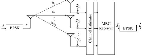
MRC is an optimum receiver combining technique for a flat fading channel with additive white Gaussian noise (AWGN) [4], used to provide NR–receiver diversity order. A schematic example of a system with MRC is shown in Figure 1.

Figure 1: Schematic example of an MRC scheme

In the transmitter, randomly generated symbols, a, are mapped using BPSK. The resulting symbols are transmitted over

R

N

h

h₁,, multipath channels. In the receiver, some AWGN respective to each receiver branch is added, namely

R

N

z

z₁,, . For a linear system, the received signal can be described in the form:

y = hs + z (7)

where y is a vector containing received symbols from each branch of the NR receiver elements, defined as: y

T NR y y

y, , , ] [ _{1 2} 

 . h _N T

R h h, , ] [ ₁ 

 is a Rayleigh

multipath fading channel defined as ([9]):



T R



L

l

j l i

i a t e i N N

h 1 _{( )} il_{, 1, ,}

0

, ,   









  (8)

Here []Tis the transpose of [], ai,lis the path gain, and



i,l is the lth phase of the multipath. Similarly, z _N T

R z z, , ] [₁

 is

the AWGNdue to the ith receiver antenna.

If the channel coefficients are perfectly available in the receiver, the detector attains optimal maximum likelihood (ML) decoding as [10]

s

sˆargmax





R N

i

i i h y P 1

, |

( s)

2

1 2 *

1 *

2 1 Re

min

arg h y s h s

R

R N

i i N

i i i

s 

   

       

   

    

  







 

(8a)

where P







  

 _{ }

 2

exp 1 ,

|hS y hS

y



. The term

2 hs y

symbols have equal energy, thus the bias energy term in (8a) is dropped [11] so that [10]:

                



 * 1 * Re min arg

ˆ h y s

s R N i i i s (8b)

where

 

* is the conjugate of

 

 . The optimal decision rule linearly combines the received signals through different diversity branches after co-phasing and weighting them with their respective channel gains. If an equivalent channel is known, the MRC rule becomes [10, 12]

i N i i N i

i s hz

h s R R





            1 * 1 2 ˆ (9)

Although affected byh*, the noise terms are still Gaussian.

The effective instantaneous SNR with MRC is



N_1R 2

i hi , where



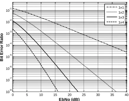
is the average SNR per antenna branch. It can be seen that the SNR of NRbranch diversity with MRC is the sum of the instantaneous SNRs for each branch. In [2], it

was shown that BER

 

_1/



NR_{as presented in Figure 2}

(BER is the bit error ratio).

Figure 2: BER performance of BPSK system for MRC with an increasing number of antennas.

The plot in Figure 2 shows that an MRC system does not act as a single element with NR times greater SNR. Due to the fact that independent faded symbol copies are received on each antenna branch, the slope of the BER changes as NR increases (but falls off exponentially).

Thus from Figure 2, the MRC combining diversity technique provides significant improvement as the number of receiver antennas increases.

2.3 Orthogonal Space Time Block Codes

Space time block coding or STBC was introduced to improve the performance of multi-antenna systems over

constrained bandwidth. It achieves full diversity and a full spatial rate (Rs) over two antenna spaces, for example [13],

S _        _* 1 * 2 2 1 s s s s (10)

In (10), there are two antenna spaces (NT) and two time slots (T) so that Rs = NT /T = 1. The symbol s provides two antenna spaces, h1 and h2. In the first time slot, s1 and s2 will be transmitted over h1 and h2, respectively. Similarly, in the second timeslot s*₂ and s₁* will be transmitted overh1and h2, respectively. Thus, in the receiver,

                       2 1 * 1 2 * 2 1 2 2 1 1 2 1 z z s h s h s h s h y y (11)

It is easier for the receiver to decouple the information- bearing symbol if an equivalent virtual channel matrix (EVCM) to the orthogonal codes of (10) can be constructed. Thus, we take the conjugate of the second row of signal received in the second timeslot in (11),

                                            * 2 1 2 1 * 1 * 2 2 1 * 2 1 1 * 2 2 * 1 2 2 1 1 * 2 1 z z s s h h h h z z s h s h s h s h y y (12)

In a linear form, (12) can be rewritten as y hvs z   _{ } , where  y



 

T

y

y₁, *₂ , s



s1,s2



Tand z



 

T

z z₁, *₂

 . H_v is the channel, usually referred to as EVCM;

v H _        _* 1 * 2 2 1 h h h h (13)

In the receiver, the STBC code permits linear decoding as

z H s H H y

H_vH _vH _v _vH

where H_vH is the Hermitian transpose of H_v. Then

v H v H

H 



2_i1h_i2 I₂ is the power gain, where I₂is a (2×2) identity matrix. Thus, the rows and columns of EVCM of the Alamouti code are orthogonal. The receiver decouples the transmitted signals s1 and s2. Using EVCM simplifies the implementation of the STBC scheme and also reduces the receiver complexity.

2.3.1 Maximum Likelihood for STBC Detection

It is assumed that channel state information (CSI) is known to the receiver. Thus, the channel coefficients h1 and h2 can be used in the decoding for a ML detector [14]. The detector is optimum if the ML detector can find the codewords



sˆ₁,sˆ₂



that minimize the Euclidean distance metric between the estimated received codeword pairs and transmitted codewords



s₁,s₂



. In STBC, the Euclidean distance metric for ML decoding is [11, 15]





_*2

1 2 * 2 1 2 2 2 2 1 1 1 2

1,s y hs h s y hs hs s

d       ₍₁₄₎

0 5 10 15 20 25 30 35 40

The joint conditional PDF of y1 and y2 given the channels h1 and h2 over which the codewords s1 and s2 are transmitted can be expressed as [11]









          2 2 1 2 2 1 2 1 2 1 2 , exp 2 1 , , , | ,   s s d s s h h y y P (15)

where 2 is the variance of z1 and z2; these are equal for uncorrelated Gaussian random variables. To reduce the

computational complexity in the detector, y₁2 y₂2terms

that are not required in the decision will be dropped. Then expanding (15), it is found that













   

1 2

2 * 1 2 2 2 * 1 2 2 * 1 2 2 1 1 * 1 2 1 2 1 2 2 , s d s d s h y s h y s s h y s h y s s s d h h             (16)

where _h h₁2 h₂2.

For PSK symbols, signal points in the constellation have

equal energy. Thus, the bias energy terms ( s₁2_hand

h

s₂2 ) are ignored; the optimum ML detection further

simplifies to

 





 

2



1* 2 2 2 1* 2



* 1 2 2 1 1 * 1 1 s h y s h y s d s h y s h y s d psk psk       (17)

Only PSK symbols will be considered in this study.

2.3.2 MIMO-STBC

Suppose that there are NR receiver antennas. Thus, each of h1 and h2 can be treated respectively as a vector of the form:

 1

h _N T

R h h

h ]

[ _{11 21}  ₁

 2

h _N T

R h h

h ]

[ _{12 22}  ₂

(18)

We know that if the equivalent channel can be derived, then the MRC when there are NR maximum receiving elements becomes [12]  r



 R N i 1 i H v y H i   r



 R N i 1



H H



s

i i v H v 

+



 R N i 1 i H v z H i  (19)

In all cases of NR, _i

i v H v H

H is an identity matrix multiplied

(as in the case NR = 1) by the channel gains such as

 

NjR1 i hi j 2

1 2

, . The noise term is rather amplified by

H vj

H , j1,,N_R. The degree of impact of H

vj

H on the

noise term impacts the closeness of the Euclidean distance metric in the receiver; this depends on the fading of the channel. The complexity in the decoupling of the

transmitted message in the receiver reduces to finding only 

s



s1,s2



T.

2.4

Quasi-orthogonal Space Time Block

Codes

A major limitation in the use of STBC is that NT > 2 is not supported. QOSTBC is a class of STBC that removes the two-transmit antenna limitation.

2.4.1 Standard QOSTBC

Standard QOSTBC achieves a full spatial rate but not full diversity [16]. In [11, 15, 17, 18], different methods for constructing QOSTBC have been described. QOSTBCs are STBCs with NT > 2 and timeslots T = 2, 4 and 8 with complex entries; STBC codes with Rs = NT/T = 1 are said to attain a full rate [11, 19].

An example of a full rate (Rs = 1) STBC code with NT = 4 and T = 4 is given as [19, 20]

           _* 12 * 34 34 12 S                  * 1 * 2 2 1 * 3 * 4 4 3 * 3 * 4 4 3 * 1 * 2 2 1 s s s s s s s s s s s s s s s s (20a)

where Ω represents the standard Alamouti STBC [21],

         _* 1 * 2 2 1 12 s s s s

and _

        _* 3 * 4 4 3 34 s s s s (20b)

(20) is an example of QOSTBC. The rate of full-diversity codes is R_s 1 [22]. Unfortunately, standard QOSTBC codes do not attain full diversity and also do not permit linear processing due to coupling terms which lie off the leading diagonal of the detection matrix [20, 23].

As seen in (20), there are h 



h₁ h₂ h₃ h₄



T antenna spaces. Combining QOSTBC from (20) with the channel vector for NR = 1,

                                                      4 3 2 1 * 1 4 * 2 3 * 3 2 * 4 1 2 4 1 3 4 2 3 1 * 3 4 * 4 3 * 1 2 * 2 1 4 4 3 3 2 2 1 1 4 3 2 1 z z z z s h s h s h s h s h s h s h s h s h s h s h s h s h s h s h s h y y y y (21)

As with Alamouti STBC codes, EVCM can be formulated by taking the conjugates of the second and fourth rows in the received matrix, thus













































































































* 4 3 * 2 1 4 3 2 1 * 1 * 2 * 3 * 4 2 1 4 3 * 3 * 4 * 1 * 2 4 3 2 1 * 4 3 * 2 1

z

z

z

z

s

s

s

s

h

h

h

h

h

h

h

h

h

h

h

h

h

h

h

h

y

y

y

y

In compact form, (22) is of (7) form except that

 y







T

y y y

y₁, *₂, ₃, ₄* ,s



s₁,s₂,s₃,s₄



Tandz



z₁,z*₂,z₃,z*₄



T. The EVCM therefore becomes

 4 v H                 * 1 * 2 * 3 * 4 2 1 4 3 * 3 * 4 * 1 * 2 4 3 2 1 h h h h h h h h h h h h h h h h (23)

Definition 1: The Equivalent Virtual Channel Matrix, hv, is

a matrix that satisfies



N_ i 1 hi

2

D, where D is a sparse

matrix with ones on its leading diagonal and at least N2/2 zeros at its off-diagonal positions; its remaining ( self-interference) entries are bounded in magnitude by 1.

In the receiver, the EVCM can be used to simplify decoding. For instance, let the decoding method proceed as:

z H s D s z H s h H y H s H v H v v H v H v                4 4 4 4 4 4 ˆ ˆ (24)

where D4 is the detection matrix for NT=4 and NR=1in the form,                  1 0 0 0 1 0 0 1 0 0 0 1 4 4 4     _h v H v H H D (25)

D4 is a Grammian matrix withh in the leading diagonal of the D4 (NT × NT) matrix; ₁ ,

2



  NT

i i

h h

 i1,,N_T is the channel power/gain.

On the other hand, h

 

  and _

      _     h h h h h 

 ₂ 1 3 2 4 _.

β is the self-interfering term that limits full-diversity performance expected of this type of QOSTBC systems. Alternative channel estimation for linear receivers, such as zero-forcing (ZF) [24], compensates for the β-term except for the noise elements. This yields sub-optimal results.

2.4.2 Interference-Free QOSTBC

Independently, two different researchers have proposed an interference-free QO-STBC; one method involves the use of Givens rotations [25] while the other uses eigenvalues [20, 23]. Both of these methods yield similar results. However, the eigenvalues approach is less complex and this will be reviewed in brief.

Definition 2 - If

A



 

a_ij is a square matrix and x is a column matrix (xi); if Axvix, where v is a scalar, then vi

is an eigenvalue and xi is an eigenvector. xi can be formed

into a square matrix





T N

x x

M ₁,, usually called a modal matrix. If the eigenvalue of A is the leading diagonal of a matrix V, then V = viI; both A and V share the same

eigenvalues, I is an identity matrix. It follows that VM

AM .

The goal of the eigenvalue computation is to eliminate the interfering terms. If A represents D4, then D4M= MV. Thus, M -1D4M = V; this is the principle of diagonalizing a matrix [26]. It follows that V contains the required diagonal terms of the diagonal matrix, viI, with no interference terms

.

Recall the decoding matrix of (25): its modal matrix from 

 M D

M 1 4 viI is

               1 0 1 0 0 1 0 1 1 0 1 0 0 1 0 1 4 v H M (26) 4 v H

M will be post-multiplied by the EVCM (

4

v

H ) for

linear decoding in the receiver, such as

4 4 hv v M

h

H 

                                      1 * 3 4 * 2 4 2 3 1 3 * 1 4 * 2 4 2 3 1 * 3 * 1 2 * 4 2 4 1 3 3 * 1 4 * 2 4 2 3 1 h h h h h h h h h h h h h h h h h h h h h h h h h h h h h h h h ₍₂₇₎

Thus, assuming a linear system of (7) form as, yHsz.

If, at the receiver, we have

z H s H H y

HH H  H (28a)

HHH can be verified to permit linear decoding with no interfering terms, β, as follows

                          1 0 0 0 0 1 0 0 0 0 1 0 0 0 0 1 h H _H H (28b)

Notice that HHH provides

4 4 4 4 1 v

v v H

H v

H H H M

M . With

ML detection, the receiver finds



sˆ₁,,sˆ₄



whose Euclidean distance metric is closest to the transmitted symbols



s₁,,s₄



.

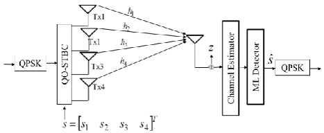
transmitted over antenna spaces h₁, h₂, h₃ and h₄, as shown in Figure 3.

Figure 3: Architecture for Implementing QOSTBC

To enable QOSTBC, EVCM is constructed as (27) for 4×1 transmission; for 3×1 design, h4 is set to zero. Noise terms (AWGN) are generated and added to each receiver branch respective to the transmitting branch. In the receiver, the linear decoding shown in (28) is performed to estimate the transmitted signals.

It is assumed that the channel state information (CSI) is known; the ML detection method is said to be optimum to find the transmitted data as [14]:

2 min

arg

ˆ y Hu

u u



  ,

where u is the transmitted data and

u

ˆ

is the estimate. The receiver finds



sˆ₁,,sˆ₄



whose Euclidean distance metric is closest to the transmitted symbols



s₁,,s₄



. This is an optimization (minimization) problem of the form

2 min

arg ˆ

F s

s H y

s  

 



(29)

where sˆ is the estimated signal vector. If s



s₁,,s₄



were transmitted and sˆ



sˆ₁,,sˆ₄



are received, then the error matrix is e



s₁sˆ₁,,s₄sˆ₄



. The fading channel is quasi-static for four consecutive timeslots; however, the noise terms are uncorrelated and statistically independent,

with zero-mean and variance



2. It follows that the probability that sˆs was detected is [27]

P(ssˆ|H) _   

  

2 SNR k

Q (30)

where



 _

      

 _x t dt

x Q

2 exp 2

1 ) (

2

 is the complementary

error function, k He2_F is the Euclidean distance metric at the receiver and SNR is the ratio of transmitted and received powers per antenna. From the Chernoff upper bound [28], the pairwise error probability (PEP) approximates to

 ˆ| )

(s s H 

  

       

  

4 exp 2

SNR k SNR

k

Q (31)

where 2 2 2

F F F H e

He  , U trace

 

UHU

F 

2

and

 

H is a Hermitian transpose of

 

 .

2.4.3 MIMO-QOSTBC

The maximum achievable diversity level for an NT × NR

MIMO system is NTNR [11], where NT is the number of

transmit elements and NR is the number of receiver

elements. In the ML detection case, the error matrix is 

e



s₁sˆ₁,,s₄sˆ₄



, then the rank of E_i,j e_i,je_iH_,j is κ and its nonzero eigenvalues are

 

_l . QOSTBC systems attain full diversity, when κ = NT.

As in the STBC case, if there are NR maximum receiver elements, then



R



 R N

i1

i H i y

H 



R



 R N

i 1



H_iHH_i



s 





R N

i1

i H i z

H 

(31)

For an i.i.d Gaussian channel with many receiver elements (e.g. NR), the average Chernoff bound simplifies to [27]

P(ssˆ)

R

T

N

N E

SNR

I 

 

 

   

 

   

  _ 

4 det

1

R N

l l

SNR

   

 

   

 

   

   









1

2

4 1

1

(32)

A major performance degradation in this case arises from

the error matrix or _l2 in the estimated noise power which is amplified byHH.

An advantage in this case (interference-free QOSTBC)

accrues from the gain contributed by HHH which amplifies the amplitude of the received signals. This varies depending on the eigenvalue (

T N i

v_1,, ) from 

 M D

M 1 ₄ V. At high SNR, where SNR/41, the error probability is bounded as [11]

P(ssˆ) R

R N

N

l l

SNR 



 





              





4

1

(33)

The idea of using the rank criterion is to attain maximum possible diversity, NTNR. The nonzero eigenvalue term,

however, provides information about the coding gain.

3. Simulation Results and Discussion

scheme as a method for MIMO transmission with STBC and QOSTBC schemes. Assuming a Raleigh fading channel, the receiver is equipped with the full knowledge of the channel state information and the antennas are reasonably separated to avoid correlation.

Figure 4: Comparison of Standard and Interference-free (Int-free) QOSTBC

To investigate a 3×1 QOSTBC design, the fourth antenna element is nulled (i.e., h4 = 0). The process for 4×1 QOSTBC implementation is then repeated for 3×1 QOSTBC. In Figure 4, it is observed that interference-free (Int-free) QOSTBC achieves about 2 dB gain with respect to the standard QOSTBC for both 4×1 QOSTBC and 3×1 QOSTBC. The gain results from the elimination of the interfering terms described above.

3.1 Simulation of STBC and QOSTBC

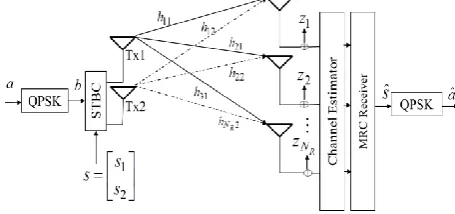
To simulate the MIMO-STBC case, some 7×105 random input symbols, a, are generated and mapped using QPSK. The resulting symbols are demultiplexed intos₁, and s₂ so that they can be transmitted over antenna spaces h₁ and h₂, as shown in Figure 5.

Figure 5: Architecture for Implementing STBC

Since there are NR receiver antennas, each of h1 and h2 is treated respectively as a vector as in (18). In the receiver, the received information on each branch is demodulated and the

channel detection performed. The information received from respective branches is combined by MRC. The resulting symbol sˆ is demapped using QPSK. For other mapping orders, such as 8-PSK, 16-PSK, 32-PSK and 64-PSK, only QPSK has been substituted in Figure 5. The results are first compared with the data in [21]. The results in Figure 6 are comparable to those reported in Figure 4 of [21] for 2×1 and 2×2 MIMO systems.

Figure 6: Results of 2×1 and 2×2 MIMO using STBC for the BPSK system

Similar to the STBC simulation case in Figure 5, QOSTBC is enabled after generating random symbols. The resulting symbols are demultiplexed intos₁, s₂, s₃ and s₄so that they can be transmitted over antenna spaces h₁, h₂, h₃ and

4

h . For MIMO-QOSTBC, each h₁, h₂, h₃ and h₄ is treated respectively as a vector of up to NR receiver antennas. In the receiver, the channel is compensated. The information detected across each antenna branch is combined with another using MRC, then using QPSK, the received symbol estimate is demapped.

3.2 Simulation of SM

Similarly, to simulate the MIMO for the SM case, some n×105 random input symbols (where n is from (2)), a, are generated and mapped using QPSK to yield b; this is the two-dimensional signal modulation. SM is a third dimension added to the default two-dimensional signal modulation. SM

maps the symbols into a table of s_CNTL_{, where C}NTL

is an NT×L matrix with complex entries. NT here denotes that there are NT possible transmitting branches provided by the SM design. In each column of the matrix, only one element is nonzero which corresponds to the antenna index that can be activated at that time. The symbol corresponding to the selected branch is transmitted over the channel, and AWGN is added. The channel estimation proceeds and the antenna index that will be used to predict the transmitted information is derived.

0 5 10 15 20 25 30

10-5 10-4 10-3 10-2 10-1 100

EbN0 (dB)

B

it

E

rr

o

r

R

a

ti

o

Traditonal QOSTBC (4x1) Int-free QOSTBC (4x1) Traditional QOSTBC (3x1) Int-free QOSTBC (3x1)

0 5 10 15 20 25

10-5 10-4 10-3 10-2 10-1 100

EbN0 (dB)

B

it

E

rr

o

r

R

a

ti

o

3.3 Results and Discussions

The results are compared for all transmitter diversity schemes. For a fair comparison, the channel and noise terms are made similar. However, the mapping scheme orders vary but permit equally likely data rates. In [29], we discussed the cases of SM and STBC for up to an NR = 4 MIMO system and QOSTBC for only to NR = 2. In this study, we include QOSTBC for up to an NR = 4 MIMO system.

A. Comparison of Analytical and Simulation Results

To validate our results we show first a comparison of analytical and simulation results with the standard QO-STBC in Figure 7.

Figure 7: Performance comparison of analytical and simulation results

The simulation results shown in Figure 7 are for a 4×1 QOSTBC diversity scheme. It can be found that the simulation result of eQOSTBC and the analytical result of eQOSTBC reasonably agree up to about 10-4.5 BER, where both results perfectly aligned. The variation at the start of the plot can be attributed to the parameter setting. Meanwhile, the interference terms in the detection matrix of the standard QOSTBC degrade its performance. Hence, the eQOSTBC outperforms the standard QOSTBC both analytically and in simulations. Both results of eQOSTBC outperform the standard QOSTBC scheme by about 2 dB, for instance, at 10-4.5 BER.

B. Two Bits Transmission

For further evaluations, we transmit two bits using SM, STBC and QOSTBC. The two bits from the SM scheme are provided by two transmit antennas and the BPSK scheme sequel to nlog₂(N_T)m of (2) with four receiving elements. On the other hand, the two bits for STBC and QOSTBC are consequent on (1). The results are shown in Figure 8. At relatively low transmission power, it is found from Figure 8 that transmitting with 2 antennas and receiving with 4 antennas for the STBC scheme is better by some 1 dB at 10-2 BER than transmitting with 4 antennas

and receiving by 4 antennas using the QOSTBC scheme. Increasing the transmission power thus improves the performance of QOSTBC up to 7.5 dB where both schemes performed equally; further increase in power however shows better performance for QOSTBC than for STBC.

Figure 8: Comparison of two bits transmissions using SM, STBC and QOSTBC

The interfering terms (β) discussed in (25) and then eliminated in (28b) impact the signal amplitude as they affect the gain _h. The results here show that results can be improved by simply increasing the transmission power. However, comparing the results of QOSTBC and SM schemes, it is found that the QOSTBC scheme outperforms the SM by about only 9 dB at 10-3 BER and then by about 11 dB at 10-5 BER. This would increase for increased symbol lengths.

C. Three Bits Transmission

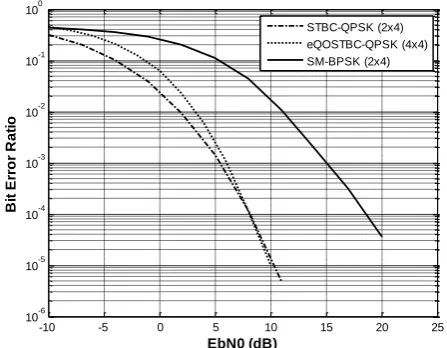
In Figure 9, we compare the results of the SM, STBC and QOSTBC schemes for three bits transmission. The three bits transmission investigation is typical of those reported in Figure 3 of [6].

Figure 9: Comparison of three bits transmissions using SM, STBC and QOSTBC

0 5 10 15 20 25

10-5 10-4 10-3 10-2 10-1 100

EbN0 (dB)

B

it

E

rr

o

r

R

a

ti

o

Traditional QO-STBC (4x1) Analy-eQOSTBC (4x1) Sim-eQOSTBC (4x1)

-10 -5 0 5 10 15 20 25

10-6 10-5 10-4 10-3 10-2 10-1 100

EbN0 (dB)

B

it

E

rr

o

r

R

a

ti

o

STBC-QPSK (2x4) eQOSTBC-QPSK (4x4) SM-BPSK (2x4)

-10 -5 0 5 10 15 20 25

10-6 10-5 10-4 10-3 10-2 10-1 100

EbN0 (dB)

B

it

E

rr

o

r

R

a

ti

o

As in [6], it can be seen that transmitting on 2 antennas and receiving on 4 antennas using the SM scheme for QPSK is better than transmitting on 4 antennas and receiving on 4 antennas using BPSK by about 1 dB. On the other hand, comparing the STBC and QOSTBC schemes, it is found that 4×4 QOSTBC performs better than 2×4 of the 8PSK scheme by about 3 dB at 10-5 BER. Then comparing them with the SM scheme, it is found that both STBC outperform SM scheme (2×4-QPSK) by about 6 dB at 10-5 BER while QOSTBC outperforms SM scheme (2×4-QPSK) by about 8 dB respectively. The benefit of the discussed QOSTBC scheme is its ability to attain full diversity and a full spatial rate resulting from the elimination of the coupling terms.

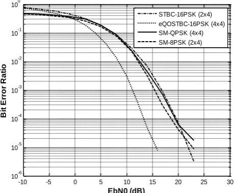
D. Four Bits Transmission

Again, we compare the performance of STBC and QOSTBC with the SM scheme when four bits are transmitted. The results are shown in Figure 10. Both 4×4-QPSK and 2×4-8PSK SM schemes perform similarly with 2×4-16PSK of STBC at 10-2 BER although with a performance marginally better than STBC. On the other hand, 4×4-16PSK QOSTBC clearly outperforms the other schemes at 10-3 BER by about 4 dB, for example.

Figure 10: Comparison of four bits transmissions using SM, STBC and QOSTBC

E. Six Bits Transmission

Finally, transmitting six bits using SM is investigated as in [6] and [8]. We then compare the results with that of transmitting six bits with the STBC and QOSTBC schemes. The results are shown in Figure 11.

In agreement with references [6] and [8], Figure 11 clearly shows that using the SM schemes to transmit six bits is more economical, in terms of transmission power, than using the STBC scheme. However, SM shows improved performance as the signal modulation order increases. The SM scheme transmission of six bits using 4×4-16PSK outperforms 2×4-32PSK progressively. On the other hand, comparing the

QOSTBC and SM schemes, the 4×4-64PSK of the QOSTBC scheme outperforms all other SM schemes and the STBC scheme. Specifically, the 4×4-64PSK QOSTBC scheme outperforms the best performing SM (16PSK that uses 4×4 antennas) among all SM schemes of six bits transmission, by about 3 dB at 10-4 BER.

Figure 11: Comparison of six bits transmissions using SM, STBC and QOSTBC

F. Evaluation of QO-STBC for NR Receivers

The interference-free QOSTBC provides information into the performance of the scheme with an increasing number of receivers, as shown in Figure 12.

Figure 12: Evaluation of receiver diversity order for NR QOSTBC system

While the SM performance improvement stems largely from the mapping scheme rather than on the number of transmitting antennas, the QO-STBC scheme exploits the diversity gain of the transmitting antennas spaces when compared to the STBC scheme. For instance, in Figure 12,

-10 -5 0 5 10 15 20 25 30 10-6

10-5 10-4 10-3 10-2 10-1 100

EbN0 (dB)

B

it

E

rr

o

r

R

a

ti

o

STBC-16PSK (2x4) eQOSTBC-16PSK (4x4) SM-QPSK (4x4) SM-8PSK (2x4)

0 5 10 15 20 25 30

10-6 10-5 10-4 10-3 10-2 10-1 100

EbN0 (dB)

B

it

E

rr

o

r

R

a

ti

o

STBC-64PSK (2x4) eQOSTBC-64PSK (4x4) SM-16PSK (4x4) SM-32PSK (2x4)

-10 -5 0 5 10 15 20 25

10-4 10-3 10-2 10-1 100

B

it

E

rr

o

r

R

a

ti

o

EbN0 (dB)

it is observed that as the number of the receiving antennas increases, the diversity gain increasingly diminishes for both mapping schemes shown (QPSK and 16PSK). The self-interfering terms (β) in (25) even though eliminated in (28) further impact the true gain_h.

However, mobile nodes are not suited (in terms of size and battery life) in supporting a large number of antennas, for example, and the slope of the 4×2 MIMO BER plot reflects appreciable space and time coding gain better (in terms of difference between NR = 2 and 1 compared to NR = 3 and 2) than the rest NR = 3 and 4. Thus, interference-free QOSTBC is an excellent technique for MIMO configuration in modern and future wireless communication applications. It transfers the complexity of the multiple antenna design algorithm from the receiver to the transmitter; transmitters, such as base stations, are more flexible in supporting complex algorithms than the receivers (such as mobile devices). By EVCM, the QOSTBC scheme studied simplifies the decoupling of the transmitted information in the receiver.

4. Conclusion

In this study, three different diversity schemes for MIMO systems were studied. These schemes include spatial modulation, STBC and QOSTBC. In the study, we explored the performance of these diversity techniques at low and relatively high spectral efficiencies. Most QOSTBC studies emphasise performance improvement with different code structures; here we implemented the scheme to include receiver diversity using MRC. Up to 4×NR can be implemented and only 4×4 QOSTBC with MRC has been investigated. The study showed that over all, the MIMO QOSTBC (for instance 4×4) scheme performed better than SM while the MIMO-STBC technique performed worst at relatively high spectral efficiency but best at low spectral efficiency. From the study, it can be said that the strength of the SM diversity scheme is in the signal modulation order, that is, the performance of the SM diversity scheme improves as the signal modulation order increases up to four bits transmission (as investigated above). At relatively low spectral efficiency (e.g. up to four bits transmission), the modulation order (with lower transmitter antenna diversity) mostly impacted the performance of the SM scheme while at relatively high spectral efficiency (e.g. at six bits transmission), lower modulation (against higher modulation order) was improved by more transmitter antenna diversity. Notwithstanding, using the QOSTBC scheme with four receiver antennas, the performance of the SM diversity scheme is poorer. Finally, where a higher signal modulation order is required, then a higher number of transmitting elements must be preferred.

Acknowledgement

This work was supported partially by TSB UK under grant application KTP008734, and financial support from Ebonyi State Government Scholarship Scheme of Nigeria.

References

[1] T.-T. Tran, Y. Shin, and O.-S. Shin, "Overview of enabling technologies for 3GPP LTE-advanced," EURASIP Journal on Wireless Communications and Networking, vol. 2012, issue 1, pp. 1-12, 2012.

[2] R. S. Adve. Receiver Diversity. Available: http://www.comm.utoronto.ca/~rsadve/Notes/DiversityReceive.pdf [3] G. L. Stüber, Principles of mobile communication: Springer, 2011. [4] K. L. Du and M. N. S. Swamy, Wireless communication systems: from

RF subsystems to 4G enabling technologies: Cambridge University Press, 2010.

[5] M. Di Renzo, H. Haas, and P. M. Grant, "Spatial modulation for multiple-antenna wireless systems: a survey," IEEE Communications Magazine, vol. 49, issue 12, pp. 182-191, 2011.

[6] R. Mesleh, H. Haas, C. W. Ahn, and S. Yun, "Spatial modulation-a new low complexity spectral efficiency enhancing technique," in First International Conference on Communications and Networking in China, 2006. ChinaCom'06. 2006, pp. 1-5.

[7] J. Jeganathan, A. Ghrayeb, L. Szczecinski, and A. Ceron, "Space shift keying modulation for MIMO channels," IEEE Transactions on Wireless Communications, vol. 8, issue 7, pp. 3692-3703, 2009. [8] R. Y. Mesleh, H. Haas, S. Sinanovic, C. W. Ahn, and S. Yun, "Spatial

modulation," IEEE Transactions on Vehicular Technology, vol. 57, , issue 4, pp. 2228-2241, 2008.

[9] A. Goldsmith, Wireless communications: Cambridge university press, 2005.

[10] T. M. Duman and A. Ghrayeb, Coding for MIMO Communication Systems: Wiley Online Library, 2007.

[11] J. Proakis and M. Salehi, Digital Communications, Fifth ed. Asia: McGraw-Hill, 2008.

[12] B. Badic, M. Rupp, and H. Weinrichter. (2005, Quasi-orthogonal space-time block codes: approaching optimality. Proc. EUSIPCO European Signal Processing Conference, Antalya, Turkey, Sept. 2005. [13] K. Anoh, O. Ochonogor, R. Abd-Alhameed, S. Jones, and T. Mapuka,

"Improved Alamouti STBC multi-antenna system using hadamard matrices," Int'l J. of Communications, Network and System Sciences, vol. 7, No. 3, pp. 83 - 89, 2014.

[14] L. Jacobs and M. Moeneclaey, "Exact BER Analysis for Alamouti’s Code on Arbitrary Fading Channels with Imperfect Channel Estimation," in Proc. 1st COST 2100 Workshop MIMO and Cooperative Communications, Trondheim-Norway, 2008, pp. 1 - 5. [15] H. Jafarkhani, Space-time coding: theory and practice: Cambridge

university press, 2005.

[16] W. Su and X.-G. Xia, "Signal constellations for quasi-orthogonal space-time block codes with full diversity," IEEE Transactions on Information Theory, vol. 50, issue 10, pp. 2331-2347, 2004.

[17] V. Tarokh, H. Jafarkhani, and A. R. Calderbank, "Space-time block codes from orthogonal designs," IEEE Transactions on Information Theory, vol. 45, issue 5, pp. 1456-1467, 1999.

[18] K. Anoh, Y. Dama, R. Abd-Alhameed, and S. Jones, "A Simplified Improvement on the Design of QO-STBC Based on Hadamard Matrices," Int'l J. of Communications, Network and System Sciences, vol. 7, issue 01, pp. 37 - 42, 2014.

[19] O. Tirkkonen, A. Boariu, and A. Hottinen, "Minimal non-orthogonality rate 1 space-time block code for 3+ Tx antennas," 2000 IEEE Sixth International Symposium on Spread Spectrum Techniques and Applications, vol. 2, pp. 429-432, 2000.

[20] Y. A. S. Dama, R. A. Abd-Alhameed, S. M. R. Jones, H. S. O. Migdadi, and P. S. Excell, "A NEW APPROACH TO QUASI-ORTHOGONAL SPACE-TIME BLOCK CODING APPLIED TO QUADRUPLE MIMO TRANSMIT ANTENNAS," Fourth International Conference on Internet Technologies & Applications, Wrexham – UK, Sept. 2011, 2011.

[21] S. M. Alamouti, "A simple transmit diversity technique for wireless communications," IEEE Journal on Selected Areas in Communications, vol. 16, issue 8, pp. 1451-1458, 1998.

[22] H. Jafarkhani, "A quasi-orthogonal space-time block code," IEEE Transactions on Communications, vol. 49, issue 1, pp. 1-4, 2001. [23] Y. Dama, R. Abd-Alhameed, T. Ghazaany, and S. Zhu, "A New

[24] B. Badic, "Space-time block coding for multiple antenna systems," PhD Thesis, Vienna University of Technology, Austria, 2005. [25] U. Park, S. Kim, K. Lim, and J. Li, "A novel QO-STBC scheme with

linear decoding for three and four transmit antennas," IEEE Communications Letters, vol. 12, issue 3, pp. 868-870, 2008. [26] K. A. Stroud and D. J. Booth, Advanced engineering mathematics:

Palgrave macmillan, 2003.

[27] S. Sandhu, R. Nabar, D. Gore, and A. Paulraj, "Introduction to Space-Time codes," Applications of Space-Time Adaptive Processing, IEE Publishers http://www.stanford.edu/group/sarg/sandhu062503.pdf (Accessed on 18/07/2015), 2003.

[28] K. Levchenko. Chernoff Bound Available: http://cseweb.ucsd.edu /~klevchen/techniques/chernoff.pdf (Accessed on 14/03/2014). [29] K. O. O. Anoh, Y. A. S. Dama, H. M. AlSabbagh, E. Ibrahim, R. A.