Meshfree methods for computational fluid dynamics
P. Niedoba1,a, L. ˇCerm´ak1, and M. J´ıcha1
1Faculty of Mechanical Engineering, Brno University of Technology, Technick´a 2896/2, 616 69 Brno, Czech Republic
Abstract. The paper deals with the convergence problem of the SPH (Smoothed Particle Hydrodynamics) meshfree method for the solution of fluid dynamics tasks. In the introductory part, fundamental aspects of mesh-free methods, their definition, computational approaches and classification are discussed. In the following part, the methods of local integral representation, where SPH belongs are analyzed and specifically the method RKPM (Reproducing Kernel Particle Method) is described. In the contribution, also the influence of boundary conditions on the SPH approximation consistence is analyzed, which has a direct impact on the convergence of the method. A classical boundary condition in the form of virtual particles does not ensure a sufficient order of consistence near the boundary of the definition domain of the task. This problem is solved by using ghost particles as a boundary condition, which was implemented into the SPH code as part of this work. Further, several numerical aspects linked with the SPH method are described. In the concluding part, results are presented of the application of the SPH method with ghost particles to the 2D shock tube example. Also results of tests of several parameters and modifications of the SPH code are shown.
1 Introduction
Currently, fluid dynamics problems are solved mostly by traditional numerical methods, such as FDM, FVM or FEM. The common feature of these methods is the use of a la-grangian mesh or eulerian grid in the domain discretiza-tion process. However, for some types of problems these methods are suited poorly. Problems in question are espe-cially those with an extreme deformation, a moving bound-ary or a free surface. The complications arising while solv-ing these problems result from the use of a mesh or a grid. And so the idea of meshfree methods evolves naturally, first being used in 1977 by Lucy L.B. [1] and Gingold R.A. & Monaghan J.J. [2]. Specifically, it was the SPH method applied to astrophysical problems of modeling the move-ment of stars and space objects.
The main idea of meshfree methods lies in modeling of the domain through field nodes without any informa-tion about relainforma-tions between these nodes. Consequently, function approximation is performed with the help of field nodes in support domains.
2 Meshfree methods
A definition of meshfree methods according to [3] is fol-lowing: a method used to create a system of algebraic equa-tions for the entire domain without using a predefined mesh for the domain discretization is defined as a meshfree me-thod.
a e-mail:[email protected]
2.1 Solution procedure
The procedure of meshfree methods consists of four basic steps:
– domain representation – function approximation – formation of system equations – solving the global equations
2.1.1 Domain representation
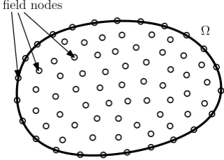
First, the domain and its boundary is modeled (not dis-cretized!) using sets of arbitrarily distributed nodes (see figure 1) in the domain and its boundary. The nodal dis-tribution is usually not uniform. The density of nodes de-pends on the accuracy requirement of the analysis. Because the nodes carry the values of a field variable (e.g. density, velocity, etc), they are often calledfield nodes. Further in the text, a field variable will be refered to as afield func-tion.
field nodes
Ω
Fig. 1.Domain representation
EPJ Web of Conferences DOI: 10.1051/
C
Owned by the authors, published by EDP Sciences, 2013 ,
epjconf 201/
01068 (2013)
45
34501068
2.1.2 Function approximation
The field functionuat any point atx=(x, y) within the do-main is approximated using the values at its nodes within the “small” local domain of the pointx, i.e.
u(x)= n
∑
i=1
ϕi(x)ui (1)
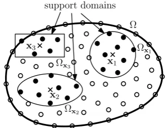
wherenis the number of nodes included in a local domain of the point atx,ui is the nodal field function at thei−th node in the local domain, andϕi(x) is theshape function of thei−th node. The “small” local domain of xwill be called thesupport domainof xand denotedΩx. The size
of support domain defines the number of field nodes ap-proximatingx. Some possible shapes of support domains are shown in figure 2.
x1
x3
x2
support domains
Ω
Ω x1
Ω x2 Ω
x3
Fig. 2.Support domains (spherical is the most common one)
2.1.3 Formation of system equations
System equations can be formulated using the shape func-tions and strong or weak formulation. These equafunc-tions are assembled into the global system matrices for the entire problem domain. For static problems, the global system equations are a set of algebraic equations. For general dy-namics problems, it is a set of differential equations.
2.1.4 Solving the global equations
The last step depends on the type of equations (algebraic, differential, etc). Note that the global equations for compu-tational fluid dynamics problems are basically nonlinear.
2.2 Classification
Meshfree methods will be classified according to the func-tion approximafunc-tion schemes [3]. Finite integral representa-tion methods include SPH - Smoothed Particle Hydrody-namics method and RKPM - Reproducing Kernel Particle Method. Finite series representation methods include MLS - Moving Least Square, PIM - Point Interpolation Method, and FPM - Finite Point Method. The last category is called the finite differential representation methods and includes GFDM - General Finite Difference Method.
This paper details two of these methods - SPH and RKPM - that fall into the first category listed above.
3 SPH method
The smoothed particle hydrodynamics method belongs to basic meshfree methods. It is used for solving partial dif-ferential equations. A system of ordinary differential equa-tions is produced after approximation of unknown func-tions (field function) and their spatial derivatives. This sys-tem is most often solved by explicit numerical methods.
3.1 Formulation
Function approximation of the field functionu(x) is based on an integral representation of the function and is given by the equation
<u(x)>=
∫
Ωx
u(ξ)W(x−ξ,h)dξ (2)
whereW(x−ξj,h)is theweight function(smoothing func-tion, kernel function),hbeing thesmoothing length, which defines the size of the support domainΩx, i.e. the
smooth-ing length determines the number of particles approximat-ing the function atx. The weight function is usually chosen to be an even function and it satisfies number of conditions, e.g. thenormality condition
∫
Ωx
W(x−ξ,h)dξ=1. (3)
Equation (2) is usually referred to askernel approximation, orSPH approximationof functionu(x).
For practical calculation, the equation (2) must be dis-cretized as follows
<u(x)>= n
∑
j=1
u(ξj)W(x−ξj,h)mj
ρj (4)
wheremjandρjare mass and density of the j−th particle inΩx. Equation (4) is called aparticle approximationof
field functionu(x).
Note that the approximation (4) corresponds to the ap-proximation (1) introduced for a general meshfree method. The shape function in this case has the form of
ϕj(x)=W(x−ξj,h)mj
ρj. (5)
Approximation of the spatial derivatives of the field function can be obtained by replacing the functionu(x) in equation (2) with its spatial derivative∇ ·u(x). Using the per-partes, the Green theorem and a discretization we ob-tain a particle approximation of the spatial derivative of the field function in the form of
<∇ ·u(x)>= n
∑
j=1
u(ξj)∇xW(x−ξj,h)
mj
ρj (6)
where∇xW(x−ξj,h) is the spatial derivative of the weight
function with respect to the variablex.
3.2 Consistency
To ensure the convergence of meshfree method, it is nec-essary that the method satisfies certain order of consis-tency. Consistency is closely related to the reproduction of polynomials.
If an approximation can exactly reproduce polynomials of degreek, i.e.
<f(x)>= f(x) (7) wheref(x) is a polynomial of degreek, than we say that the approximation hask-th order of consistency, i.e.Ck consis-tency.
Specifically, consistency of the SPH approximation (4) is given by the following definition. The SPH approxima-tion hasCkconsistency if and only if weight functions sat-isfy the condition
∫
Ωx
ξlW(x−ξ,h)dξ=xl for l=0,1, . . . ,k. (8)
It can be shown thatC0 consistency follows directly from the normality condition (3), which is a necessary con-dition for the weight functions. Thus the SPH approxima-tion has alwaysC0consistency.
Furthermore, we can prove the theorem, which says that the SPH approximation hasC1consistency if and only if hasC0consistency and also the appropriate weight func-tion is an even funcfunc-tion.
We see that the order of consistency depends only on the properties of weight functions.
3.3 Boundary treatment
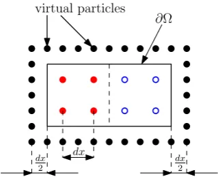
The issue of boundary conditions is generally very diffi -cult in the SPH method. We answer the question of prop-erly defining the boundary condition that prevented par-ticles from escaping out of the domain. Furthermore, we discuss consistency near the boundary of the domain (near boundary area).
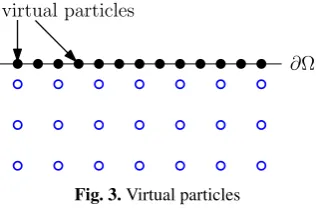
3.3.1 Virtual particles
The first approach is the use of virtual particles. These par-ticles are situated on the boundary and by repulsive force acting on the particles in the near boundary area (near boundary particles). Hence, virtual particles prevent an un-physical penetration through the boundary.
∂Ω virtual particles
Fig. 3.Virtual particles
Unfortunately, this approach violates the condition for C1consistency of the SPH approximation in the near boun-dary area. This fact is due to the undesirable “cutting off”
of the weight function support, see figure 4. Thus, the ap-propriate weight function is not an even function.
x W
i j
Wi Wj ∂Ω
Fig. 4.Example of a 1D task, particle jis situated in the near boundary area
3.3.2 Ghost particles
A much better way is to use ghost particles as a boundary condition. In contrast to virtual particles, this approach cre-ates a dynamic wall that is constructed at each time step. Ghost particles are formed symmetrically (according to the boundary) to the near boundary particles as “twin” parti-cles, see figure 5.
∂Ω ghost particles
vτf
vnf vf
vτ
vn v
Fig. 5.Ghost particles, velocities are formed symmetrically (slip wall)
Using ghost particles ensures C1 consistency of the SPH approximation, because the shape functions of the near boundary particles can be even functions.
3.4 RKPM method
The reproducing kernel particle method belongs to the cat-egory of finite integral methods, and is a modification of the SPH method. This method adds the so-called correc-tion funccorrec-tion to the SPH formulacorrec-tion to ensure certain or-der of consistency. The particle approximation of the func-tionu(x) is defined as
<u(x)>= n
∑
j=1
u(ξj)C(x,ξj)W(x−ξj,h)mj ρj (9)
whereC(x,ξ) is thecorrection function.
Note that the approximation (9) corresponds to the ap-proximation (1), where the shape function has the form of
ϕj(x)=C(x,ξ)W(x−ξj,h)mj
4 Shock tube 2D problem
In this section we show the results of the shock tube prob-lem in 2-dimensions (2D) depending on the boundary con-ditions described in section 3.3.
The shock tube problem is a good numerical bench-mark that shows the ability of numerical methods to deal with discontinuities. In addition, we know the exact so-lution of this problem in 1D and therefore we can com-pare it with the results of the 2D task. These results were obtained using a program based on the SPH method. The program was written in theFortranprogramming language (Intel(R) Visual Fortran Compiler Professional 11.1.067) in the MS Visual Studio 2008 IDE for .NET Framework v. 3.5. The basis was the source code from the book [4]. Post-processing, i.e. graphs of particular variables was realized using thematlabsoftware v. 7.11.0 (R2010b).
4.1 Description of the shock tube 2D problem
It is the examination of the phenomenon which occurs in the rectangular container after removal of an imaginary barrier. This barrier separates two different (density, pres-sure and energy) fluids. After removing the barrier, we will observe the spread of a shock wave, a rarefaction wave and a contact discontinuity.
4.2 Initial settings
The initial conditions were taken from (L. Hernquist, 1989, [5]) for 1D problem, which has been extended to 2D, in this way
ρL=1, pL=1, vL=0, ρR=0.25, pR=0.1795, vR=0
where the subscripts LandR denote the fluid on the left and right side of the barrier. Assume that both fluids satisfy properties of an ideal gas, therefore the initial values of the internal energyeare calculated from the equation of state. So we haveeL=2.5 andeR=1.795.
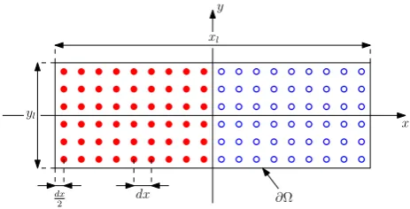
In the simulation 3200 particles were used. Specifi-cally, 320 inx-direction and 10 iny-direction. The sizes of the domain (container) arexl=0.8 andyl=0.025. Spac-ing between particles is constant withdx=dy=2.5·10−3. The center of the container is placed at the origin of the co-ordinate system (x=y=0). The distribution of particles is shown in figure 6, which is only illustrative due to the large number of particles.
Boundary condition is set as the slip wall and the end time of the simulation was set tot=0.2 s.
4.3 Parameter settings
The shock tube problem is generally a very fast phenome-non, therefore it can be assumed that it is very sensitive to the parameter settings. This assumption have been demon-strated by testing. To achieve the “correct” setting of these parameters, much effort is usually required.
Now we show the parameter settings for the shock tube 2D problem, which has been obtained by a number of tests.
dx
dx
2
x y
yl
xl
∂Ω
Fig. 6.Initial distribution of particles
Weight function: The exponential weight function has been used for the shock tube problem. The disadvantage of this approach is a global discontinuity at the boundaries of the support domains. The exponential function has derivatives of all orders, which has a positive effect on the stability of the solution. When testing other weight functions (cubic spline, quintic spline), there were significant oscillations in the solution.
Artificial viscosity: The artificial viscosity was used to re-move the oscillations which originated in areas of discon-tinuities. It is a component that is added to the pressure terms of the Euler equations or Navier-Stokes equations.
Variable smoothing length: Due to the variable density of particles, the variable smoothing length is required to pre-serve an almost constant number of particles in particular support domains during the approximation.
Nearest Neighboring Particle Searching (NNPS): Because of the large number of particles and the variable smooth-ing length, the tree method was used as a search algorithm.
Time step: To ensure the stability of the shock tube prob-lem, a sufficiently small time step is necessary. After the tests, the time step was set todt=0.0005 and for achieving the simulation end time (t=2), 400 steps were required.
Boundary conditions: In section 3.3, we have shown that the SPH method in conjunction with virtual particles does not satisfy theC1consistency condition at the near bound-ary area. This problem was corrected by using ghost parti-cles as a boundary condition.
Now we show the implementation problems and their solutions in the application of these boundary conditions.
• Virtual particles: We solved the problem how to set the repulsive force large enough to prevent particles es-cape out of the domain, and small enough to avoid degradation of the solution by acting of this force. It is therefore a compromise which could not be found for the classical location of these particles (on the domain boundary). We have to solve this problem by moving the virtual particles outside of the domain as shown in figure 7. This approach allowed us to set a repulsive force that prevents particles from escaping out of the domain and is small enough.
virtual particles
dx
2 dx
dx
2 ∂Ω
Fig. 7.Corrected position of virtual particles
domain extension (bydx) in each coordinate direction. If there was a strict requirement to preserve the domain size then it would be necessary to change the disposi-tion of particles, i.e. the number of particles or their spacing.
• Ghost particles: In this case, we discussed how to set the properties and position of ghost particles that are created in adition to particles located at the domain cor-ners. Using [6], the position of ghost particles has been resolved. Thus, three ghost particles are always created to the particles at each corner of the domain, as shown in figure 8.
∂Ω ghost particles
v2f
v
v3f
v1f
i f1
i
f2
i
f3
i
Fig. 8.Positions and velocities of ghost particles, which are cre-ated to particleisituated at the domain corner
We have also solved the problem how to properly set the mass of these ghost particles. The best variant was to choose the same mass as particlei, which also corresponds to the text [7].
4.4 Simulation results
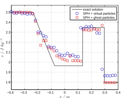
The simulation was performed for both types of bound-ary conditions, i.e. first for virtual particles only, and than for ghost particles only. Ghost particles were implemented into the SPH code within this work. Figures 9, 10, 11 and 12 show the progressions of axial velocity, density, pres-sure and internal energy in the longitudinal section, i.e. y=0. The solid line shows the exact solution of the Euler equations for a 1D task.
It can be seen that the solution obtained with the help of ghost particles captures the shape of the exact solu-tion better than a solusolu-tion that uses virtual particles. We
−0.4 −0.3 −0.2 −0.1 0 0.1 0.2 0.3 0.4
0 0.1 0.2 0.3 0.4 0.5 0.6 0.7 0.8
x / m
v
/
m
s
−
1
exact solution SPH + virtual particles SPH + ghost particles
Fig. 9.Axial velocity, longitudinal section,t=0.2 s
−0.4 −0.3 −0.2 −0.1 0 0.1 0.2 0.3 0.4
0.2 0.3 0.4 0.5 0.6 0.7 0.8 0.9 1
x / m
ρ
/
k
g
m
−
3
exact solution SPH + virtual particles SPH + ghost particles
Fig. 10.Axial density, longitudinal section,t=0.2 s
−0.4 −0.3 −0.2 −0.1 0 0.1 0.2 0.3 0.4 0.1
0.2 0.3 0.4 0.5 0.6 0.7 0.8 0.9 1
x / m
p
/
N
m
−
2
exact solution SPH + virtual particles SPH + ghost particles
Fig. 11.Axial pressure, longitudinal section,t=0.2 s
−0.4 −0.3 −0.2 −0.1 0 0.1 0.2 0.3 0.4 −0.05
0 0.05
x / m
y
/
m
Fig. 13.Position of particles,t=0.2 s
−0.4 −0.3 −0.2 −0.1 0 0.1 0.2 0.3 0.4
1.8 1.9 2 2.1 2.2 2.3 2.4 2.5
x / m
e
/
J
k
g
−
1
exact solution SPH + virtual particles SPH + ghost particles
Fig. 12.Axial internal energy, longitudinal section,t=0.2 s
located aroundx=0.13. Slight deviations from the exact solution of both simulations, especially in the rarefaction wave area, are probably caused by the continuity method used for the calculation of density. The continuity method does not preserve mass exactly, but is able to deal with the discontinuity.
Figure 13 shows the specific location of particles at the end of the simulation in the case of using ghost par-ticles. We can also notice the relation between the number of ghost particles and the density of fluid particles distri-bution. The number of ghost particles is reduced in areas where the fluid particles are closer. This is due to decreas-ing smoothdecreas-ing length in areas with greater density of par-ticle distribution. This is necessary in order to preserve an almost constant number of particles in each support do-main. Similarly, we obtain that the number of ghost par-ticles increases in the places where the fluid parpar-ticles are closer. Figure 14 shows the detail of the contact disconti-nuity area aroundx=0.13.
5 Conclusion
This paper covers our work on the convergence problem of the SPH method. The classical form of boundary condi-tion, i.e. virtual particles, does not preserveC1consistency of the SPH approximation in the near boundary area. This negative feature has a direct impact on convergence and thus also on the accuracy of the method. This problem has been solved by using ghost particles as a boundary con-dition. This type of particles has been implemented to the SPH code. The previously described theory was demon-strated on the 2D shock tube example. The SPH method with ghost particles expressed the form of the exact
solu-0.08 0.1 0.12 0.14 0.16 0.18
−0.04 −0.03 −0.02 −0.01 0 0.01 0.02 0.03 0.04
x / m
y
/
m
Fig. 14.Position of particles, the detail of the contact discontinu-ity area,t=0.2 s
tion better than the SPH method with virtual particles. We have confirme the influence ofC1consistency of the SPH approximation on the accuracy of the method. Especially in the near boundary area.
6 Acknowledgements
This research was funded by Brno University of Technol-ogy, Faculty of Mechanical Engineering through the project number FSI-S-11-6.
References
1. L.B. Lucy, Astronomical Journal82, (1977) 1013-1024 2. R.A. Gingold, J.J. Monaghan, Monthly Notices of the
Royal Astronomical Society181, (1977) 375-389 3. G.R. Liu,Mesh Free Methods: Moving beyond the
Fi-nite Element Method(CRC Press, Boca Raton, 2002) 4. G.R. Liu, M.B. Liu,Smoothed Particle Hydrodynamics
- a meshfree particle method(World Scientific Publish-ing, New Jersey, 2003)
5. L. Hernquist, N. Katz, The Astrophysical Journal Sup-plement Series70, (1989) 419-446
6. A. Colagrossi, G. Colicchio, D. Le Touz´e, Proc. 2nd SPHERIC Workshop2, (2007) 59-62
7. S. Børve, Proc. 6th SPHERIC Workshop6, (2011) 313-320