Rare event sampling with stochastic growth algorithms
Thomas Prellberg1,a
School of Mathematical Sciences, Queen Mary University of London Mile End Road, London E1 4NS, United Kingdom
Abstract. We discuss uniform sampling algorithms that are based on stochastic growth methods, using sampling of extreme configurations of polymers in simple lattice mod-els as a motivation. We shall show how a series of clever enhancements to a fifty-odd year old algorithm, the Rosenbluth method, led to a cutting-edge algorithm capable of uniform sampling of equilibrium statistical mechanical systems of polymers in situa-tions where competing algorithms failed to perform well. Examples range from collapsed homo-polymers near sticky surfaces to models of protein folding.
1 Introduction
A large class of sampling algorithms are based on Markov Chain Monte Carlo methods [1]. Here we shall introduce an alternative method of sampling based on stochastic growth methods. Stochastic growth means that one attempts to randomly grow configurations of interest from scratch by succes-sively increasing the system size (usually up to a desired maximal size).
For simplicity, we shall restrict ourselves to the setting of lattice path models of linear polymers, that is, models based on random walks configurations on a regular lattice, such as the square or the simple cubic lattice. If we impose self-avoidance, i.e. if we forbid those random walk configurations that repeatedly visit the same lattice site, we obtain the model of Self-avoiding Walks (SAW), used to describe polymers in a good solvent. Monte-Carlo Simulations of SAW have been proposed as early as 1951 [2]. Extensions of SAW have been used to study a variety of different phenomena, such as polymer collapse, adsorption of polymers at a surface, and protein folding.
While this setting is rich enough to allow for the simulation of physically relevant scenarios, it is also simple enough to serve as the ideal background for the description of the particular class of stochastic growth algorithms which we shall describe here.
In Section 2 we briefly discuss simple sampling of SAW, review Rosenbluth sampling as the basic algorithm, and by combining this with pruning and enrichment strategies, discuss the Pruned and Enriched Rosenbluth Method (PERM), and its extension to uniform sampling, flatPERM. In Section 3 we conclude with a description of an extension of stochastic growth methods to settings beyond linear polymers, called Generalized Atmospheric Rosenbluth Method (GARM).
2 Sampling of Self-Avoiding Walks
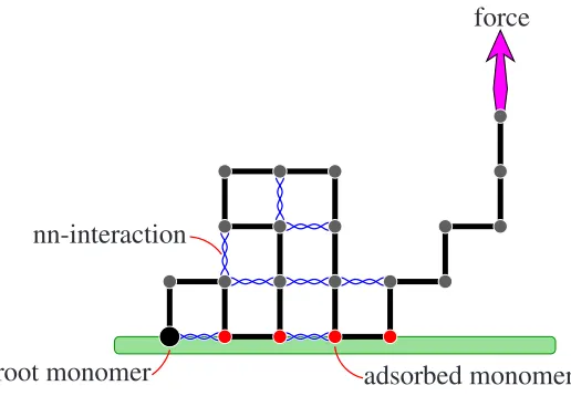
In this section we want to consider the simulation of self-avoiding random walks (SAW), i.e. random walks obtained by forbidding any random walk that contains multiple visits to a lattice site. SAW is the canonical lattice model for polymers in a good solvent. Moreover, it forms the basis for more realistic models of polymers with physically and biologically relevant structure, as indicated in Figure 1.
a e-mail:[email protected] C
Owned by the authors, published by EDP Sciences, 2013
adsorbed monomer
root monomer
force
nn-interaction
Fig. 1.A lattice model of a polymer tethered to a sticky surface under the influence of a pulling force.
However, the introduction of self-avoidance turns a simple Markovian random walk without mem-ory into a complicated non-Markovian random walk; when growing a self-avoiding walk, one needs to test for self-intersection with all previous steps, leading to a random walk with infinite memory.
2.1 Simple Sampling
Algorithm 1Simple Sampling of Self-Avoiding Walk
s·←0
S amples←0
whileS amples<MaxS amplesdo
S amples←S amples+1 n←0, Start at origin s0←s0+1
whilen<MaxLengthdo
Draw one of the neigboring sites uniformly at random
ifOccupiedthen
Reject entire walk and exit loop
else
Step to new site n←n+1 sn←sn+1
end if end while end while
It is straight-forward to generate SAW by simple sampling. Generating ann-step self-avoiding walk with the correct statistics, i.e. such that every walk is generated with the same probability, is equivalent to generatingn-step random walks and reject those random walks that self-intersect. Al-gorithm 1 accomplishes this by generating two-dimensional random walks and rejecting thecomplete configuration when self-intersection occurs.
At each step, the walk has four possibilities to continue, and chooses one of these with probability p = 1/4. Therefore an estimator for the total number of n-step SAW after S samples have been generated is given by 4ns
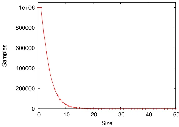
Generating SAW with simple sampling is very inefficient. There are 4n n-step random walks, but only about 2.638n n-step self-avoiding walks on the square lattice. The probability of successfully generating ann-step self-avoiding walk therefore decreases exponentially fast, leading to very high attrition1. Longer walks are practically inaccessible, as seen in Figure 2.
0 200000 400000 600000 800000 1e+06
0 10 20 30 40 50
Samples
Size
Fig. 2.Attrition of started walks generated with Simple Sampling. From 106started walks none grew more than 35 steps.
2.2 Rosenbluth Sampling
A slightly improved sampling algorithm was proposed in 1955 by Rosenbluth and Rosenbluth [3]. The basic idea is to avoid self-intersections by only sampling from the steps that lead to self-avoiding configurations. In this way, the algorithm only terminates if the walk is trapped in a dead end and can-not continue growing. While this still happens exponentially often, Rosenbluth sampling can produce substantially longer configurations than simple sampling.
While simple sampling generates all configurations with equal probability, configurations gener-ated with Rosenbluth sampling are genergener-ated with different probabilities. To understand this in detail, it is helpful to introduce the notion of anatmosphereof a configuration; this is the number of ways in which a configuration can continue to grow. For one-dimensional simple random walks the atmo-sphere is always two, for two-dimensional simple random walks on the square lattice the atmoatmo-sphere is always four (and if one forbids immediate self-reversals, the atmosphere is always three except for the very first step). However, for self-avoiding walks on the square lattice the atmosphere is a configuration-dependent quantity assuming values between four (for the first step) and zero (for a trapped configuration that cannot be continued). We shall denote the atmosphere of a configurationφ bya(φ). If it is clear from the context, we will drop the argument and speak about the atmospherea.
If a configuration has atmospherea, this means that there areadifferent possibilities of growing the configuration, and each of these can get selected with probability p =1/a. To balance this, the
1 The algorithm can be improved somewhat by forbidding immediate reversals of the random walk, but the
weight of this configuration is therefore multiplied by the atmospherea. Ann-step walk grown by Rosenbluth sampling therefore has weight
Wn=
n−1
Y
i=0
ai,
whereai are the atmospheres of the configuration afterigrowth steps. This walk is generated with probabilityPn =1/Wn, so thatPnWn =1 as required. Algorithm 2 shows a pseudocode implementa-tion of Rosenbluth sampling.
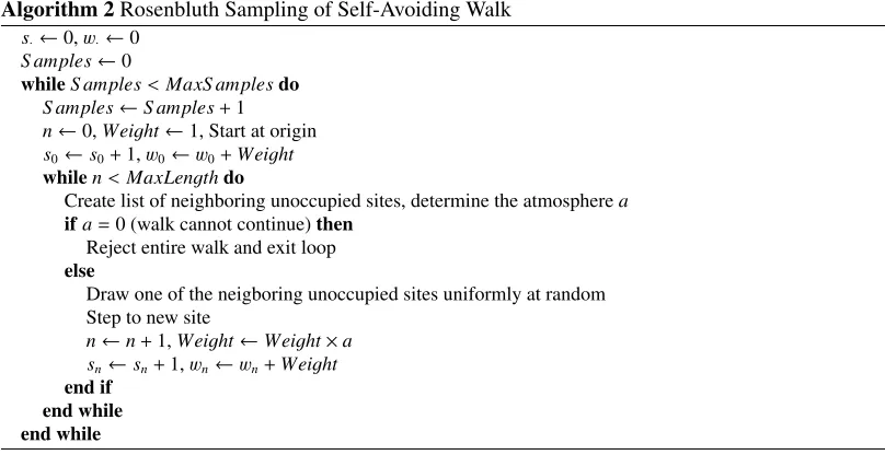
Algorithm 2Rosenbluth Sampling of Self-Avoiding Walk
s·←0,w·←0
S amples←0
whileS amples<MaxS amplesdo
S amples←S amples+1 n←0,Weight←1, Start at origin s0←s0+1,w0←w0+Weight
whilen<MaxLengthdo
Create list of neighboring unoccupied sites, determine the atmospherea
ifa=0 (walk cannot continue)then
Reject entire walk and exit loop
else
Draw one of the neigboring unoccupied sites uniformly at random Step to new site
n←n+1,Weight←Weight×a sn←sn+1,wn←wn+Weight
end if end while end while
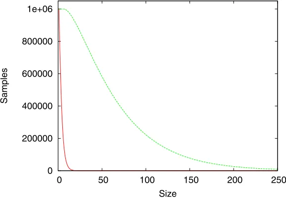
Figure 3 shows the improvement gained by Rosenbluth sampling over simple sampling.
2.3 Pruned and Enriched Rosenbluth Sampling
It took four decades before Rosenbluth sampling was improved upon. In 1997 Grassberger augmented Rosenbluth sampling with pruning and enrichment strategies, calling the new algorithm Pruned and Enriched Rosenbluth Method, or PERM [4]. There are a variety of pruning and enrichment strategies that are possible, and the strategies used in [4] were somewhat different from the ones we shall describe now. For alternate versions and enhancements we also refer to [5] and references therein.
Suppose a walk has been generated that has weightwas opposed to a target weightW. In the ideal situationwis equal toW as desired. If that is not the case, either the weightwis to small, i.e. the ratio R=w/W <1, or the weightwis too large, i.e.R=w/W >1. In the first case we will employ pruning, i.e. we will probabilistically remove walks.
– IfR =w/W <1, continue growing with probabilityRand weightwset toW, and stop growing with probability 1−R.
In the second case we will employ enrichment, i.e. we will continue to grow multiple copies of the walk.
0 200000 400000 600000 800000 1e+06
0 50 100 150 200 250
Samples
Size
Fig. 3.Attrition of started walks generated with Rosenbluth Sampling compared with Simple Sampling. Walks with a few hundred steps become accessible.
While we chose to describe pruning and enrichment as different strategies, note that enrichment pro-cedure is actually identical to the pruning propro-cedure ifR<1: whenbRc=0 then enrichment reduces to making 1 copy with probabilityRand 0 copies with probability 1−R, which is just the pruning procedure.
Whereas in simple (or Rosenbluth) sampling the generated walks are each grown independently from length zero, pruning and enrichment leads to the generation of a large tree-like structure of more or less correlated walks grown from one seed. We call the collection of these walks a tourof the algorithm. The tree structure of a tour allows for successively growing all copies obtained during the enrichment in a natural way.
Pruning and enrichment can be incorporated quite easily as follows. repeat
ifzero atmosphere or maximal length reachedthen set number of enrichment copies to zero
else
prune/enrich step: compute number of enrichment copies end if
ifnumber of enrichment copies is zerothen prune: shrink to previous enrichment end if
ifconfiguration shrunk to zerothen start new tour
store data for new configuration else
decrease number of enrichment copies ifpositive atmospherethen
grow new step
store data for new configuration end if
end if
Note that in case of constant atmosphere this reduced precisely to the pruned and enriched sam-pling for simple random walks encountered earlier. Algorithm 3 contains a more detailed pseudo-code version of PERM for self-avoiding walks.
Algorithm 3Pruned and Enriched Rosenbluth Sampling of Self-Avoiding Walks
s·←0,w·←0
T ours←0,n←0,Weight0←1 Start new walk with step size zero a←0,Copy0←1
s0←s0+1,w0←w0+Weight
whileT ours<MaxT oursdo{Main loop}
ifn=MaxLengthora=0then{Maximal length reached or atmosphere zero: don’t grow}
Copyn←0
else{pruning/enrichment by comparing with target weight}
Ratio←Weightn/wn
p←Ratio mod 1
Draw random numberr∈[0,1]
ifr<pthen
Copyn← bRatioc+1
else
Copyn← bRatioc
end if
Weightn←wn
end if
ifCopyn=0then{Shrink to last enrichment point or to size zero}
whilen>0 andCopyn=0do Delete last site of walk n←n−1
end while end if
ifn=0 andCopy0=0then{start new tour}
T ours←T ours+1,
Start new walk with step size zero a←0,Copy0←1
s0←s0+1,w0←w0+Weight
else
Create list of neighboring unoccupied sites, determine the atmospherea
ifa>0then
Copyn←Copyn−1
Draw one of the neigboring unoccupied sites uniformly at random Step to new site
n←n+1,Weightn←Weightn×a
sn←sn+1,wn←wn+Weightn
end if end if end while
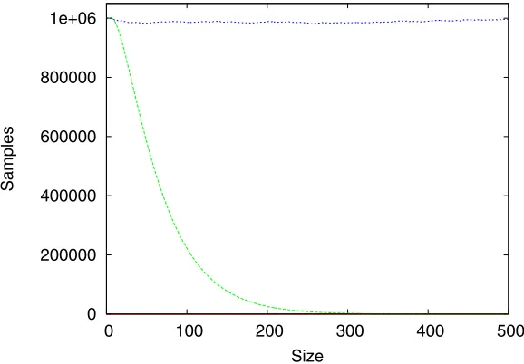
Figure 4 shows the significant improvement gained by adding pruning and enrichment strategies to Rosenbluth Sampling.
2.4 Flat Histogram Rosenbluth Sampling
0 200000 400000 600000 800000 1e+06
0 100 200 300 400 500
Samples
Size
Fig. 4.Attrition of started walks with PERM compared with Rosenbluth Sampling. In the case of PERM, a virtually constant number of samples is obtained.
ticanonical PERM [8]. This was followed by Prellberg and Krawczyk [9], who designed flatPERM, a flat-histogram version of PERM estimating directly the microcanonical density of states.
Within the context of the algorithms developed here, incorporating uniform sampling into PERM is straightforward. First we note that PERM already is a uniform sampling algorithm in system size. This is not apparent at all from the algorithm, as the guiding principle has been to adjust pruning and enrichment with respect to a target weight, not with respect to any criterion of poor local sampling. It is rather that uniform sampling is a consequence of adjusting pruning and enrichment around the desired target weight.
It is therefore reasonable (and very much in the spirit of the previous section) to extend PERM to a microcanonical version, in which configurations of sizenare separated with respect some additional parameter. One simply determines this parameter when growing the configuration and stores the data by binning with respect to this additional parameter. Then, when considering pruning and enrichment, the target weight is computed from the binned data. More precisely, if the additional parameter is calledm, storing the data is changed from
sn ←sn+1,wn←wn+Weightn
to
sn,m←sn,m+1,wn,m←wn,m+Weightn
and computing enrichment ratio is changed from Ratio←Weightn/wn
to
Ratio←Weightn/wn,m
and this is about it.
In the previous section this additional parameter has been the end-point position of the random walk. Here, we shall consider by example the case ofinteracting self-avoiding walks, where each walk configuration has an energy proportional to the number of non-consecutive nearest-neigbour contacts between occupied lattice sites.
1 100000 1e+10 1e+15 1e+20 1e+25
0 5 10 15 20 25 30 35 40
Samples and Number of States
Energy
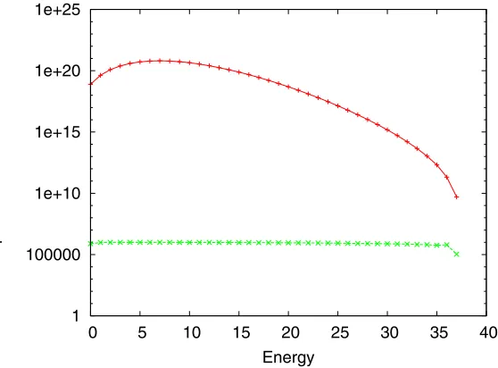
Fig. 6.Number of States of Interacting Self-Avoiding Walks with 50 steps at fixed energy estimated from 106 flatPERM tours. The lower graph shows the number of actually generated samples for each energy.
Figure 6 shows the simulation results of a simulation of interacting self-avoiding walks of up to 50 steps using 106tours starting at size zero. This led to the generation of about 106samples for each value ofmatn = 50 steps, and enabled the estimation of the number of states over ten orders of magnitude.
0 5 10
15 20 25 30 35 40 0 10 20
30 40
50 10000
100000 1e+06 1e+07
Samples
Energy
Size
0 5 10
15 20 25 30 35 40 0 10 20 30 40
50 1
100000 1e+10 1e+15 1e+20 1e+25
Number of States
Energy
Size
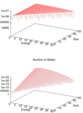
Fig. 7.Interacting Self-Avoiding Walks with up to 50 steps generated with flatPERM. The upper figure shows that a roughly constant number of samples is obtained across the whole range of sizes and energies, and the lower figure shows the estimated number of states for a given Sizenand Energym.
self-avoiding walks with up ton=1024 steps, where the density of states ranges over three hundred orders of magnitude, all obtained from one single simulation.
3 Extensions
simulation of objects that can be grown uniquely from a seed. In the case of linear polymer models, this is accomplished by appending a step to the end of the current configuration2.
However, if one wants to simulate polymers with a more complicated structure, such as branched polymers, there no longer is an easy way to uniquely grow a configuration. A lattice model for a two-dimensional branched polymer is given by lattice trees, i.e. trees embedded in the latticeZ2. For a given lattice tree it is no longer clear how it has been grown from a seed; this could have happened in a variety of ways.
3.1 Generalized Atmospheric Rosenbluth Sampling
It turns out that there is an extension to Rosenbluth sampling, called Generalized Atmospheric Rosen-bluth Method, or GARM [10], that is suitable for these more complicated growth processes. The key idea is to generalize the notion of atmosphere by introducing an additional negative atmospherea− indicating in how many ways a configuration can be reduced in size. For linear polymers the nega-tive atmosphere is always unity, as there is only one way to remove a step from the end of the walk. However, for a given lattice tree the removal of any leaf of the tree gives a smaller lattice tree, and the negative atmospherea−can assume rather large values.
Algorithm 4Generalised Atmospheric Sampling
s·←0,w·←0
S amples←0
whileS amples<MaxS amplesdo
S amples←S amples+1
n←0,Weight←1, Start with seed configuration s0←s0+1,w0←w0+Weight
whilen<MaxS izedo
Create list of growth possibilities, determine the atmospherea
ifa=0 (no growth possible)then
Reject entire configuration and exit loop
else
Draw one of the growth possibilities uniformly at random Grow configuration
n←n+1,Weight←Weight×a Compute negative atmospherea−
Weight←Weight/a−
sn←sn+1,wn←wn+Weight
end if end while end while
Surprisingly there is a very simple extension to the Rosenbluth weights discussed above. If a configuration has negative atmospherea−, this means that there area−different possibilities in which
the configuration could have been grown. An n-step configuration grown by GARM therefore has weight
Wn=
n−1
Y
i=0
ai
a−i+1 , (1)
whereaiare the (positive) atmospheres of the configuration afterigrowth steps, anda−i are the negative atmospheres of the configuration afterigrowth steps. It can be shown that the probability of growing this configuration isPn=1/Wn, so againPnWn=1 holds as required.
2 In a more abstract setting, Rosenbluth sampling has for example been used to study the number of so-called
The implementation of GARM is not any more complicated than the implementation of Rosenbluth sampling. Algorithm 2 gets changed minimally by inserting the lines
Compute negative atmospherea− Weight←Weight/a−
immediately after having grown the configuration.
While implementing GARM is quite straightforward, there generally is a need for more com-plicated data structures for the simulated objects, and one needs to find efficient algorithms for the computation of positive and negative atmospheres.
It is now possible to add pruning and enrichment to GARM, and to extend this further to flat histogram sampling, just as has been described in the previous section for Rosenbluth sampling.
For further extensions to Rosenbluth sampling, and indeed many more algorithms for simulating self-avoiding walks, as well as applications, see [5].
References
1. D. P. Landau and K. Binder,A Guide to Monte Carlo Simulations in Statistical Physics, Cambridge University Press, 2005
2. G. W. King, inMonte Carlo Method, volume 12 ofApplied Mathematics Series, National Bureau of Standards, 1951
3. M. N. Rosenbluth and A. W. Rosenbluth, J. Chem. Phys.23356 (1955) 4. P. Grassberger, Phys. Rev E563682 (1997)
5. E. J. Janse van Rensburg, J. Phys. A42323001 (2009) 6. F. Wang and D. P. Landau, Phys. Rev. Lett.862050 (2001) 7. B. A. Berg and T. Neuhaus, Phys. Lett. B267249 (1991) 8. M. Bachmann and W. Janke, Phys. Rev. Lett.91208105 (2003) 9. T. Prellberg and J. Krawczyk, Phys. Rev. Lett.92120602 (2004)