Medical Image Segmentation with Deep Learning

(1)

University of Wisconsin Milwaukee University of Wisconsin Milwaukee

UWM Digital Commons

Theses and Dissertations May 2020

Medical Image Segmentation with Deep Learning

Chuanbo Wang

University of Wisconsin-Milwaukee

Follow this and additional works at: https://dc.uwm.edu/etd Part of the Electrical and Electronics Commons

Recommended Citation Recommended Citation

Wang, Chuanbo, "Medical Image Segmentation with Deep Learning" (2020). Theses and Dissertations. 2434.

https://dc.uwm.edu/etd/2434

This Thesis is brought to you for free and open access by UWM Digital Commons. It has been accepted for inclusion in Theses and Dissertations by an authorized administrator of UWM Digital Commons. For more information, please contact [email protected].

(2)

MEDICAL IMAGE SEGMENTATION WITH DEEP LEARNING

by

Chuanbo Wang

A Thesis Submitted in Partial Fulfillment of the Requirements for the Degree of

Master of Science in Engineering

at

The University of Wisconsin-Milwaukee May 2020

(3)

ii

ABSTRACT

MEDICAL IMAGE SEGMENTATION WITH DEEP LEARNING

by

Chuanbo Wang

The University of Wisconsin-Milwaukee, 2016 Under the Supervision of Zeyun Yu

Medical imaging is the technique and process of creating visual representations of the body of a patient for clinical analysis and medical intervention. Healthcare professionals rely heavily on medical images and image documentation for proper diagnosis and treatment. However, manual interpretation and analysis of medical images is time-consuming, and inaccurate when the interpreter is not well-trained. Fully automatic segmentation of the region of interest from medical images have been researched for years to enhance the efficiency and accuracy of understanding such images. With the advance of deep learning, various neural network models have gained great success in semantic segmentation and spark research interests in medical image segmentation using deep learning. We propose two convolutional frameworks to segment tissues from different types of medical images.

Comprehensive experiments and analyses are conducted on various segmentation neural networks to demonstrate the effectiveness of our methods. Furthermore, datasets built for training our networks and full implementations are published.

(4)

iii

(5)

iv

LIST OF FIGURES

Figure 1. An illustration of images in our dataset. ... 8 Figure 2. The encoder-decoder architecture of MobilenetV2... 10 Figure 3. A demonstration of a depth-separable convolution layer compared to

an original convolution layer ... 12 Figure 4. An illustration of the segmentation result and the post-processing

method.. ... 14 Figure 5. An overview of the model architecture of the 3D segmentation network ... 16

(8)

vii

LIST OF TABLES

Table 1. Evaluation on our dataset. ... 20 Table 2. Comparison of total numbers of trainable parameters. ... 22 Table 3. Evaluation on the Medetec dataset. ... 23 Table 4. Segmentation performance of our 3D method using different

combinations of modalities as the training dataset ... 25 Table 5. Segmentation result evaluation of the conventional 3D U-Net, UNICHK,

(9)

1

Chapter 1: Introduction

For accurate diagnosis and proper treatment planning, healthcare professionals rely heavily on medical images, including computed tomography (CT) images, magnetic resonance imaging (MRI) scans, and natural images taken in clinical settings. Such images are further measured and analyzed to provide quantitative parameters in the diagnosis and treatment. Traditionally, this process is performed manually by specialists. However, this process is tedious and time-consuming given the large number of images involved for each patient. Furthermore, the shortage of medical resources and clinicians in primary and rural healthcare settings decreases the access and quality of care to millions of Americans. Consequently, research interests in automatic segmentation and measurement from medical images were captured, especially in the fields of intervertebral discs segmentation from 3D MRI scans and wound segmentation from 2D images. Such studies can be roughly categorized into two groups: traditional methods and deep learning methods.

Studies in the first group focus on combining computer vision techniques and traditional machine learning approaches. These studies apply manually designed feature extraction to build a dataset that is later used to support machine learning algorithms. [1] proposed an algorithm to segment the wound region from 2D images. 49 features are extracted from a wound image using K-means clustering, edge detection, thresholding, and region growing in both grayscale and RGB. These features are filtered and prepared into a feature vector that is used to train a

(10)

Multi-2

Layer Perceptron (MLP) and a Radial Basis Function (RBF) neural network to identify the region of a chronic wound. [2] proposed an intervertebral discs (IVD) segmentation method applied to chest MRI scans. The method solves an energy minimization problem by graph-cuts algorithms where the graph edges are divided into two types: terminal edges that connect the voxels and non-terminal edges that connect neighbor voxels. [3] proposed to generate a Red-Yellow-Black-White (RYKW) probability map of an input image with a modified hue-saturation-value (HSV) model. This map then guides the region of interest (ROI) segmentation process using either optimal thresholding or region growing. [4] and [5] applied an atlas-based method that first proposes atlas candidates as initialization and then utilize label fusion to combine IVD atlases to generate the segmentation mask. However, to generate the initialization, [4] registers IVD atlases to the localization obtained by integral channel features and a graphical parts model. Whereas [5] uses data-driven regression to create a probability map, which further defines an ROI as the initialization for segmentation. [6] demonstrated a wound segmentation method using an energy-minimizing discrete dynamic contour algorithm applied to the saturation plane of the image in its HSV color model. The wound area is then calculated from a flood fill inside the enclosed contour. Another regression-based IVD segmentation method [7] was proposed to address the segmentation of multiple anatomic structures in multiple anatomical planes from multiple imaging modalities with a sparse kernel machines-based regression. A 2D segmentation method proposed in [8] applied an Independent Component Analysis

(11)

3

(ICA) algorithm to the pre-processed RGB images to generate hemoglobin-based images, which are used as input of K-means clustering to segment the granulation tissue from the wound images. These segmented areas are utilized as an assessment of the early stages of ulcer healing by detecting the growth of granulation tissue on ulcer bed. [9] proposed a similar system to segment the burn wounds from 2D images. Cr-Transformation and Luv-Transformation are applied to the input images to remove the background and highlight the wound region. The transformed images are segmented with a pixel-wise Fuzzy C-mean Clustering (FCM) algorithm. [10] proposes an automatic method using a conditional random field (CRF) based on super-voxels generated from a variant of simple linear iterative clustering (SLIC). A support vector machine (SVM) is then used to perform super-voxels classification, which is later integrated into the potential function of the CRF for final segmentation using graph cuts. [11] builds an automatic IVD segmentation framework that localizes the vertebral bodies using regression-forests-based landmark localization and optimizes the landmarks by a high-level Markov Random Field (MRF) model of global configurations. The IVD segmentation mask is then generated from an image processing pipeline that optimizes the convex geodesic active contour based on the geometrical similarity to IVDs. In [12], IVD segmentation is performed by iteratively deforming the corresponding average disc model towards the edge of each IVD, in which edge voxels are defined by a 26-dimension feature vector including intensity, gradient orientation and magnitude, self-similarity context (SSC) descriptor, and Canny edge

(12)

4

descriptor, etc. This group of methods suffers from at least one of the following limitations: 1) As in many traditional computer vision systems, the computation complexity is high in the segmentation pipeline, 2) They depend on manually tuned parameters and empirically handcrafted features which does not guarantee an optimal result. Additionally, they are not immune to severe pathologies and rare cases, which are very impractical from a clinical perspective, and 3) The performance is evaluated on a small biased dataset.

Since the achievements AlexNet [13] accomplished in the ImageNet large scale visual recognition challenge [14] in 2012, the success of deep learning in the domain of computer vision sparked interests in semantic segmentation [15] using deep convolutional neural networks (CNN) [16]. Traditional computer vision and machine learning methods typically make decisions based on feature extraction. Thus, to find the segmentation mask, one must guess which wound features are important and then design sophisticated algorithms that capture these features. However, in CNN, feature extraction and decision making are integrated. The features are extracted by convolutional kernels and their importance is determined by the network during the training process. A typical CNN architecture consists of convolutional layers and a fully connected layer as the output layer, which requires fixed-size inputs. One successful variant of CNN is fully convolutional neural networks (FCN) [17]. Networks of this type are composed of convolutional layers without any fully connected layer at the end of the network. This enables the network to take arbitrary input sizes and prevent the

(13)

5

loss of spatial information caused by the fully connected layers in CNNs. Several FCN-based methods have been proposed to solve the wound segmentation problem. [18] estimated the wound area by segmenting wounds with the vanilla FCN architecture [17]. With time-series data consisting of the estimated wound areas and corresponding images, wound healing progress is predicted using a Gaussian process regression function model. However, the mean Dice accuracy of the segmentation is only evaluated to be 64.2%. [19] proposed to employ the FCN-16 architecture on the wound images in a pixel-wise manner that each pixel of an image is predicted to which class it belongs. The segmentation result is simply derived from the pixels classified as a wound. By testing different FCN architectures, they are able to achieve a Dice coefficient of 79.4% on their dataset. However, the network’s segmentation accuracy is limited in distinguishing small wounds and wounds with irregular borders as the tendency is to draw smooth contours. [20] proposed a new FCN architecture that replaces the decoder of the vanilla FCN with a skip-layer concatenation up-sampled with bilinear interpolation. A pixel-wise softmax layer is appended to the end of the network to produce a probability map, which is post-processed to be the final segmentation. A dice accuracy of 91.6% is achieved on their dataset with 950 images taken under an uncontrolled lighting environment with a complex background. However, images in their dataset are semi-automatically annotated using a watershed algorithm. This means that the deep learning model is learning how the watershed algorithm labels wounds as opposed to human specialists.

(14)

6

FCNs are also adopted to solve the IVD segmentation problem. [21] extends the 2D FCN into a 3D version with end-to-end learning and inference. [22] proposes a 3D multi-scale FCN that expands the typical single-path FCN to three pathways where each pathway takes volumetric regions on a different scale. Features from three pathways are then concatenated to generate a probability map, from which the final 3D segmentation mask is generated by simple thresholding. More recently, a modified FCN, U-Net [45] and its variants have outperformed the state-of-art in many biomedical image segmentation tasks. The pertinacious architecture and affluent data augmentation allow U-Net to quickly converge to the optimal model from a limited number of annotated samples. Comparing to CNN and vanilla FCN, U-Net uses skip connections between contraction and expansion and a concatenation operator instead of a sum, which could provide more local information to global information while expansion. Moreover, U-Net is symmetric such that feature maps in an expansive path facilitate to transfer more information. U-Net has been widely applied to the IVD segmentation problem. [23]applies a conventional 3D U-Net [24] on the IVD dataset provided by the 3rd MICCAI Challenge [25] of Intervertebral Discs Localization and Segmentation. [26] designs a new network architecture based on U-Net, boundary specific U-Net (BSU). The architecture consists of repeated application of BSU pooling layers and residual blocks, following the idea of residual neural networks (RNN). [27] extends the conventional U-Net by adding three identical pathways in the contracting path to process the multi-modality channels of the input. These pathways are

(15)

7

interconnected with hyper-dense connections to better model relationships between different modalities in the multi-modal input images. [28] proposes an IVD segmentation pipeline that first segments the vertebral bodies using a conventional 2D U-Net to find the spine curve and IVD centers. Transverse 2D images and sagittal 3D patches are cropped around the centers to train an RNN fusing both 2D and 3D convolutions. However, the effectiveness of data augmentation and multi-modality input images are not fully explored in these works.

To better explore the capacity of deep learning on the wound segmentation and IVD segmentation problem, we propose two frameworks to automatically segment ROI from medical images. The first framework is built above a 2D network, MobileNetsV2 [29], to tackle the wound segmentation problem. This network is light-weight and computationally efficient since significantly fewer parameters are used during the training process. We built a large dataset of wound images with segmentation annotations done by wound specialists. This is by far the largest dataset focused on wound segmentation to the best of our knowledge. The second framework proposed is built upon a 3D network, 3D U-Net [24], to segment IVD from MRI scans. We adopted a two-stage pipeline: localizing the IVDs followed by segmenting IVDs based on the localization. To examine the effectiveness of different combinations of modalities, various modalities are analyzed with respect to image properties of the input data based on our analysis in the conducted experiments.

(16)

8

Chapter 2: Dataset

2.1 The Wound Dataset

2.1.1 Dataset Construction

There is currently no public dataset large enough for training deep-learning-based models for wound segmentation. To explore the effectiveness of wound segmentation using deep learning models, we collaborated with the Advancing the Zenith of Healthcare (AZH) Wound and Vascular Center, Milwaukee, WI. Our chronic wound dataset was collected over 2 years at the center and includes 1,109 foot ulcer images taken from 889 patients during multiple clinical visits. The raw images were taken by digital single-lens reflex cameras and iPads under uncontrolled illumination conditions, with various backgrounds. Fig. 1 shows some sample images in our dataset.

The raw images collected are of various sizes and cannot be fed into our deep learning model directly since our model requires fixed-size input images. To unify the size of images in our dataset, we first localize the wound by placing bounding boxes around the wound using an object localization model we trained de novo, YOLOv3 [31]. Our localization dataset contains 1,010 images, which are also collected from the AZH Wound and Vascular Center. We augmented the images and built a training set Figure 1. An illustration of images in our dataset. The first row contains the raw images collected. The second row consists of segmentation mask annotations we create with the AZH wound and vascular

(17)

9

containing 3645 images and a testing set containing 405 images. For training our model we have used LabelImg [32] to manually label all the data (both for training and testing). The YOLO format has been used for image labeling. The model has been trained with a batch size of 8 for 273 epochs. With an intersection over union (IoU) rate of 0.5 and non-maximum suppression of 1.00, we get the mean Average Precision (mAP) value of 0.939. In the next step, image patches are cropped based on the bounding boxes result from the localization model. We unify the image size (224 pixels by 224 pixels) by applying zero-padding to these images, which are regarded in our dataset data points.

2.1.2 Data Annotation

During training, a deep learning model is learning the annotations of the training dataset. Thus, the quality of annotations is essential. Automatic annotation generated with computer vision algorithms is not ideal when deep learning models are trained to learn how human experts recognize the wound region. In our dataset, the images were manually annotated with segmentation masks that were further reviewed and verified by wound care specialists from the collaborating wound clinic. Initially only foot ulcer images were annotated and included in the dataset as these wounds tend to be smaller than other types of chronic wounds, which makes it easier and less time-consuming to manually annotate the pixel-wise segmentation masks. In the future we plan to create larger image libraries to include all types of chronic wounds, such as venous leg ulcers, pressure ulcers, and surgery wounds as well as non-wound reference images. The AZH Wound and Vascular Center, Milwaukee, WI, had consented to make our dataset publicly available.

(18)

10

2.2 The IVD Dataset

The IVD dataset [30], by courtesy of Prof. Guoyan Zheng from the University of Bern, consists of 8 sets of 3D multi-modality MRI spine images collected from 8 patients in 2 different stages of prolonged bed test. Each spine image contains at least 7 IVDs of the lower spine (T1-L5) and four modalities following Dixon protocol: in-phase (inn), opposed-in-phase (opp), fat and water (wat) images. In detail, water images are spin echo images acquired from water signals. fat images are spin echo images acquired from water signals. In-phase images are the sum of water images and fat images. Opposed-phase images are the difference between water images and fat images. In total, there are 32 3D single-modality volumes and 66 IVDs. For each IVD, segmentation ground truth is composed of binary masks manually labeled by three trained raters under the guidance of clinicians.

(19)

11

Chapter 3: Methods

3.1 Wound Segmentation

In this section we describe our method with the architecture of the deep learning model for wound segmentation. The transfer learning used during the training of our model and the post-processing methods including hole filling and removal of small noises are also described.

3.1.1 Model Architecture Overview

A convolutional neural network (CNN), MobileNetV2 [29], is adopted to segment the wound from the images. Compared with conventional CNNs, this network substitutes the fundamental convolutional layers with depth-wise separable convolutional layers [33] where each layer can be separated into a depth-wise convolution layer and a point-wise convolution layer. A depth-wise convolution performs lightweight filtering by applying a convolutional filter per input channel. A point-wise convolution is a 1 × 1 convolution responsible for building new features through linear combinations of the input channels. This substitution reduces the computational cost compared to traditional convolution layers by almost a factor of k2 where k is the convolutional kernel size. Thus, depth-wise separable convolutions are much more computationally efficient than conventional convolutions suitable for mobile or embedded applications where computing resource is limited. For example, the mobility of MobileNetV2 could benefit medical professionals and patients by

(20)

12

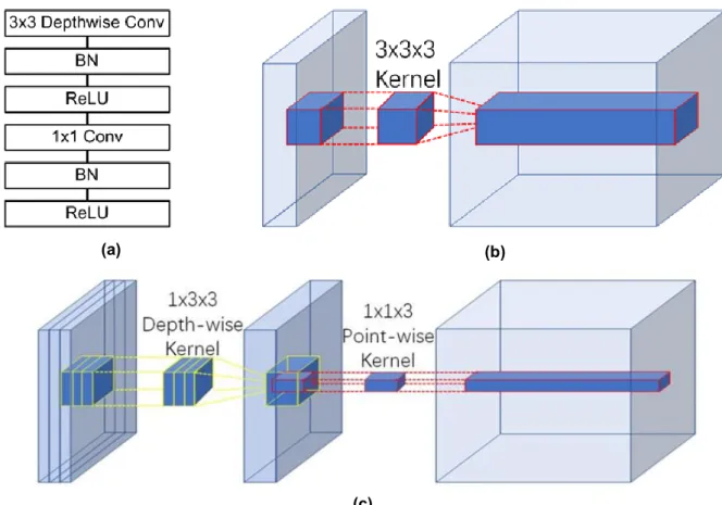
allowing instant wound segmentation and wound area measurement immediately after the photo is taken using mobile devices like smartphones and tablets. An example of a depth-wise separable convolution layer is shown in Figure 3(c), compared to a traditional convolutional layer shown in Figure 3(b).

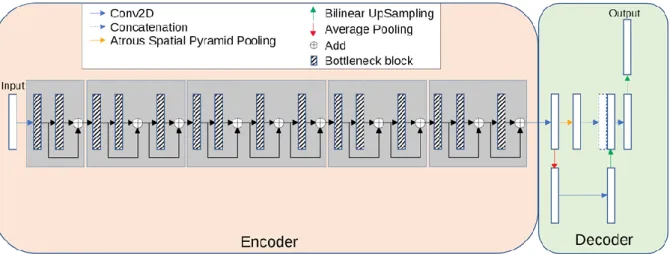
The model has an encoder-decoder architecture as shown in Figure 2. The encoder is built by repeatedly applying the depth-separable convolution block (marked with diagonal lines in Figure 2). Each block, illustrated in Figure 3(a), consists of six layers: a 3 × 3 depth-wise convolutional layer followed by batch normalization and rectified linear unit (Relu) activation [34], and a 1 × 1 point-wise convolution layer followed again by batch normalization and Relu activation. To be more specific, Relu6

(a) _(b)

(c)

Figure 3. (a) A depth-separable convolution block. The block contains a 3 × 3 depth-wise convolutional layer and a 1 × 1 point-wise convolution layer. Each convolutional layer is followed by

batch normalization and Relu6 activation. (b) An example of a convolution layer with a 3 × 3 × 3 kernel. (c) An example of a depth-wise separable convolution layer equivalent to (b).

(21)

13

[35] was used as the activation function. In the decoder, shown in Figure 2, the encoded features are captured in multiscale with a spatial pyramid pooling block, and then concatenated with higher-level features generated from a pooling layer and a bilinear up-sampling layer. After the concatenation, we apply a few 3 × 3 convolutions to refine the features followed by another simple bilinear up-sampling by a factor of 4 to generate the final output. A batch normalization layer is inserted into each bottleneck block and a dropout layer is inserted right before the output layer. In MobileNetV2, a width multiplier α is introduced to deal with various dimensions of input images. we let α = 1 thus the input image size is set to 224 pixels × 224 pixels in our model

3.1.2 Transfer Learning

To make the training more efficient, we used transfer learning for our deep learning model. Instead of randomly initializing the weights in our model, the MobileNetV2 model, pre-trained on the Pascal VOC segmentation dataset [36] is loaded before the model is trained on our dataset. Transfer learning with the pre-trained model is beneficial to the training process in the sense that the weights converge faster and better.

3.1.3 Post-processing

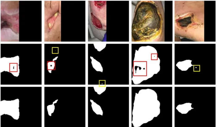
Post Processing, including hole filling and removal of small regions, is performed to improve the segmentation results as shown in Figure 4. We notice that abnormal tissue like fibrinous tissue within chronic wounds could be identified as non-wound and

(22)

14

cause holes in the segmented wound regions. Such holes are detected by finding small connected components in the segmentation results and filled to improve the true positive rate using connected component labeling (CCL) [37]. The small noises are removed in the same way. The images in the dataset are cropped from the raw image for each wound. So, we simply remove noises in the results by removing the connected component small enough based on adaptive thresholds. To be more specific, a connected region is removed when the number of pixels within the region is less than a threshold, which is adaptively calculated based on the total number of pixels segmented as wound pixels in the image.

Figure 4. An illustration of the segmentation result and the post processing method. The first row illustrates images in the testing dataset. The second row shows the segmentation results predicted by our model without any post processing. The holes are marked with red boxes and the noises are marked with yellow

(23)

15

3.2 IVD Segmentation

In our proposed 3D method, a two-stage coarse-to-fine strategy is used to tackle the segmentation problem directly on 3D volumes. The general workflow is illustrated in Fig. 3. In the first stage, each IVD is localized and a voxel is assigned as its center. These centers are used to divide the volume into small 3D patches, each of which contains a single IVD. In the second stage, a multimodal deep learning model is trained on the patches for precise segmentation.

Medical images are often complex and noisy in nature where ROI is relatively small comparing to the background. We first localize the IVDs in the image and then crop 3D patches based on the localization. This not only gets rid of some background but simplifies the problem for the segmentation stage and reduces the computational cost as well. It has been shown that 3D U-Net achieves the best localization result but not the best segmentation result [25] We use this two-stage strategy to work around this problem. In the end, post-processing is performed to generate the final segmentation.

3.2.1 Localization Network

For the localization of IVDs, we train a localization network, which is a conventional 3D U-net, on the IVD dataset to roughly locate the IVDs from the volume. From this segmentation, we have a good estimate of IVD centers by finding the center of each connected component after removing small regions.

(24)

16

From our observation, IVDs are generally sparsely located in 3D space with a distance from each other and share a common disc-like morphological profile. Thus, we simply put a 35*35*25 bounding box around each estimated center to crop a 3D patch. Then we zero-pad the patches to 36*36*28 so they can be nicely fed into the segmentation network in the next stage described below.

3.2.2 Segmentation Network

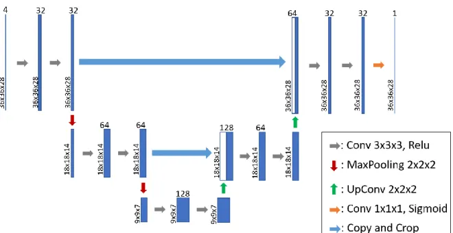
For IVD segmentation from the 3D patches, we employ a modified 3D U-Net architecture that essentially looks at IVD segmentation as a regression problem. This network takes 3D patches as input and predicts 3D patches where the intensity value on each voxel stands for how confident is the network in the voxel belonging to an IVD. Figure 5 presents an overview of the architecture of our 3D segmentation network. Each step in the contracting path consists of repeated application of two 3x3x3 unpadded 3D convolutions followed by a Relu. A dropout operation is inserted between

(25)

17

the two convolutions to reduce the dependence on the training dataset and increase the accuracy. A dropout rate of 0.2 is used following the analysis [38] on the dropout effect in CNN. We also apply batch normalization to speed up and stabilize the training process and a 2x2x2 max pooling layer with stride 2 for down-sampling after every two convolutional layers. At each down-sampling step, we double the number of feature channels. Every step in the expansive path consists of an up-sampling of the feature map followed by a 2x2x2 up convolution that halves the number of feature channels, a concatenation with the corresponding feature map from the contracting path, and two 3x3x3 convolutions, each followed by a Relu. The output layer is a 1x1x1 convolution layer with sigmoid activation used to generate the segmentation mask for each modality. In total the network has 12 convolutional layers and 1.4 million parameters.

3.2.3 Post-processing

The prediction from the segmentation stage contains 3D patches with continuous voxel intensity values that representing how confident is the network in the voxel belonging to an IVD. The final segmentation mask for each patch is obtained by binary thresholding with a threshold of 0.5, which means voxels that are predicted more likely to be IVD voxels than background voxels are included in the segmentation mask. Then the mask patches are assembled back to a 3D volume of the lower spine, with the same size of the IVD dataset, using the IVD center locations from the localization stage and zero-padding.

(26)

18

Chapter 4: Results

4.1 Wound Segmentation Results

We describe the evaluation metrics and compare the segmentation performance of our method with several popular and state-of-the-art methods. Our deep learning model is trained with data augmentation and preprocessing. Extensive experiments were conducted to investigate the effectiveness of our network. FCN-VGG-16 is a popular network architecture for wound image segmentation [19] [39]. Thus, we trained this network on our dataset as the baseline model. For fairness of comparison, we used the same training strategies and data augmentation strategies throughout the experiments.

4.1.1 2D Evaluation Metrics

To evaluate the segmentation performance, Precision, Recall, and the Dice coefficient are adopted as the evaluation metrics [40]:

Precision: Precision shows the accuracy of segmentation. More specifically, Precision measures the percentage of correctly segmented pixels in the segmentation and is computed by:

Precision = 𝑇𝑟𝑢𝑒 𝑝𝑜𝑠𝑖𝑡𝑖𝑣𝑒𝑠

𝑇𝑟𝑢𝑒 𝑝𝑜𝑠𝑖𝑡𝑖𝑣𝑒𝑠 + 𝐹𝑎𝑙𝑠𝑒 𝑝𝑜𝑠𝑖𝑡𝑖𝑣𝑒𝑠

Recall: Recall also shows the accuracy of segmentation. More specifically, it measures the percentage of correctly segmented pixels in the ground truth and is computed by:

Recall = 𝑇𝑟𝑢𝑒 𝑝𝑜𝑠𝑖𝑡𝑖𝑣𝑒𝑠

(27)

19

Dice coefficient (Dice): Dice shows the similarity between the segmentation and the ground truth. Dice is also called F1 score as a measurement balancing Precision and Recall. More specifically, Dice is computed by the harmonic mean of Precision and Recall:

Dice = 2 × 𝑇𝑟𝑢𝑒 𝑝𝑜𝑠𝑖𝑡𝑖𝑣𝑒𝑠

2 × 𝑇𝑟𝑢𝑒 𝑝𝑜𝑠𝑖𝑡𝑖𝑣𝑒𝑠 + 𝐹𝑎𝑙𝑠𝑒 𝑛𝑒𝑔𝑡𝑖𝑣𝑒𝑠 + 𝐹𝑎𝑙𝑠𝑒 𝑝𝑜𝑠𝑖𝑡𝑖𝑣𝑒𝑠

4.1.2 Experiment setup

The deep learning model in the presented work was implemented in python with Keras [41] and TensorFlow [42] backend. To speed up the training, the models were trained on a 64-bit Ubuntu PC with an 8-core 3.4GHz CPU and a single NVIDIA RTX 2080Ti GPU. For updating the parameters in the network, we employed the Adam optimization algorithm [43], which has been popularized in the field of stochastic optimization due to its fast convergence compared to other optimization functions. Binary cross entropy was used as the loss function and we also monitored Precision, Recall and the Dice score as the evaluation matrices. The initial learning rate was set to 0.0001 and each minibatch contained only 2 images for balancing the training accuracy and efficiency. The convolutional kernels of our network were initialized with HE initialization [44] to speed up the training process and the training time of a single epoch took about 77 seconds. We used early stopping to terminate the training so that the best result was saved when there was no improvement for more than 100 epochs in terms of Dice score. Eventually, our deep learning model was trained for around 1000 epochs before overfitting.

(28)

20

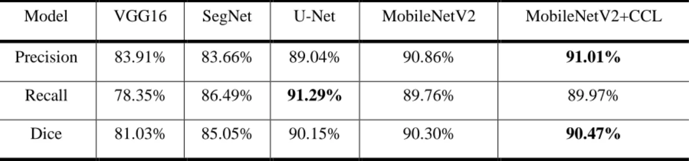
To evaluate the performance of the proposed method, we compared the segmentation results achieved by our methods with those by FCN-VGG-16 [19] [39] and SegNet [18]. We also added 2D U-Net [45] to the comparison due to its outstanding segmentation performance on biomedical images with a relatively small training dataset. The segmentation results predicted by our model are demonstrated in Figure 4 along with the illustration of our post-processing method. Quantitative results evaluated with the different networks are presented in Table 1 where bold numbers indicate the best results among all four models. To better demonstrate the accuracy of the models, the numbers shown in the table are the highest possible number reached among various trainings.

Table 1. Evaluation on our dataset.

Model VGG16 SegNet U-Net MobileNetV2 MobileNetV2+CCL

Precision 83.91% 83.66% 89.04% 90.86% 91.01%

Recall 78.35% 86.49% 91.29% 89.76% 89.97%

Dice 81.03% 85.05% 90.15% 90.30% 90.47%

4.1.3 Comparing our method to the others

In the performance measures, the highest Dice score was obtained by our MobileNetV2+CCL model. VGG16 was shown to have the worst performance among all the other CNN architectures. Our model also had the highest Precision of 94.76%, which indicates that MobileNetV2 can segment the region with most true positive pixels. The Recall of our model tested to be the second highest among all models, at

(29)

21

89.97%. This was 1.32% behind the highest Recall, 91.29%, which was achieved by VGG16. Finally, the results show that our model achieves the highest overall accuracy with a mean Dice score of 90.47%. Our accuracy was slightly better than the U-Net architecture and significantly higher than SegNet and VGG16.

Comparing our model to VGG16, the Dice score is boosted from 81.03% to 90.47% tested on our dataset. Based on the appearance of chronic wounds, we know that wound segmentation is complicated by various shapes, colors and the presence of different types of tissue. The patient images captured in clinic settings also suffer from various lighting conditions and perspectives. In MobileNetV2, the deeper architecture has more convolutional layers than VGG16, which makes MobileNetV2 more capable to understand and solve these variables. MobileNetV2 utilizes residual blocks with skip connections instead of the conventional convolution layers in VGG16 to build a deeper network. These skip connections bridging the beginning and the end of a convolutional block allows the network to access earlier activations that weren’t modified in the convolutional block and enhance the capacity of the network.

Another comparison between U-Net and SegNet indicates that the former model is significantly better in terms of mean Dice score. Similar to the previous comparison, U-Net also introduces skip connections between convolutional layers to replace the pooling indices operation in the architecture of SegNet. These skip connections concatenate the output of the transposed convolution layers with the feature maps from the encoder at the same level. Thus, the expansion section which consists of a

(30)

22

large number of feature channels allows the network to propagate localization combined with contextual information from the contraction section to higher resolution layers. Intuitively, in the expansion section or “decoder” of the U-Net architecture, the segmentation results are reconstructed with the structural features that are learned in the contraction section or the “decoder”. This allows the U-Net to make predictions at more precise locations.

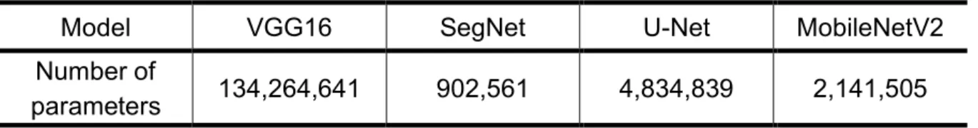
Besides the performance, our method is also efficient and lightweight. As shown in Table 2, the total number of trainable parameters in MobileNetV2 was only a fraction of the number in U-Net and VGG16. Thus, the network took less time during training and could be applied to devices with less memory and limited computational power. Alternatively, higher-resolution input images could be fed into MobileNetV2 with less memory size and computational power comparing to the other models.

Table 2. Comparison of total numbers of trainable parameters.

Model VGG16 SegNet U-Net MobileNetV2

Number of

parameters 134,264,641 902,561 4,834,839 2,141,505

4.1.4 Comparison within the Medetec Dataset

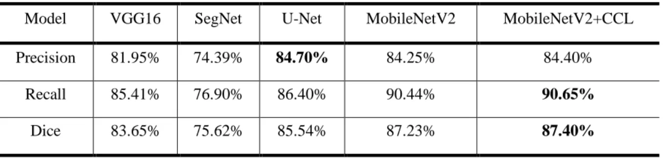
Apart from our dataset, we also conducted experiments on the Medetec Wound Dataset [46] and compared the segmentation performance of these methods. The results are shown in Table 3. We directly applied our model, trained on our dataset, to perform segmentation on the Medetec dataset as the testing dataset. The highest Dice score is evaluated to 86.95% using MobileNetV2+CCL. This performance evaluation

(31)

23

agrees with our conclusion drawn from the testing on our dataset. MobileNetV2 outperforms the other models regardless of which chronic wound segmentation dataset is used, thereby demonstrating that our model is robust and unbiased.

Table 3. Evaluation on the Medetec dataset.

Model VGG16 SegNet U-Net MobileNetV2 MobileNetV2+CCL

Precision 81.95% 74.39% 84.70% 84.25% 84.40%

Recall 85.41% 76.90% 86.40% 90.44% 90.65%

Dice 83.65% 75.62% 85.54% 87.23% 87.40%

4.2: IVD Segmentation Results

4.2.1 3D Evaluation Metrics

To evaluate the segmentation performance, two metrics are adopted from the 2015 MICCAI Challenge [25]. In addition to Dice coefficient mentioned in section 4.1.1, we also calculated the Hausdorff distance (HD) that measures the distance between two surface meshes. We compute HD for surfaces reconstructed from the ground true segmentation mask and our segmentation result. Surfaces are generated using Iso2mesh [47] from binary segmentation masks. The closest distance from each vertex on the source surface mesh to the target surface mesh is found and HD is then computed. A smaller HD value indicates better segmentation performance.

4.2.2 Effectiveness of the multi-modality data

(32)

24

images from the training dataset are more accurate and less noisy near the lower IVDs than that by the original full-modality data. Moreover, using the training dataset without in-phase images, our localization network is able to learn more details and make much more accurate predictions about the IVD centers. This makes the localization of centers more stable and allows us to simply remove small regions (marked by yellow boxes) and then crop a fix-size 3D patch for each IVD in the volume to train the segmentation network.

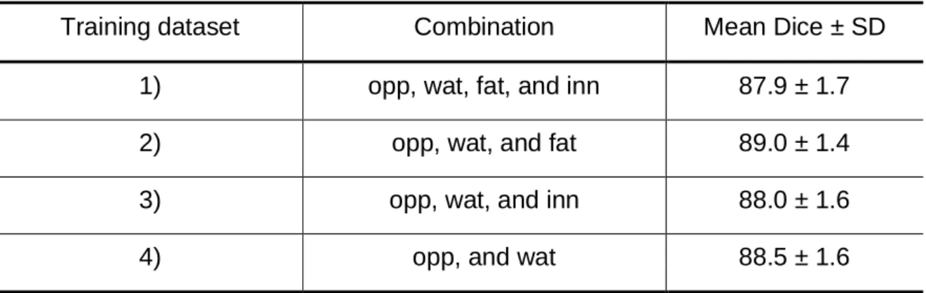
From the multi-modality analysis, we found that the fat and in-phase images have a significantly lower contrast among all the modalities. To analyze the effectiveness of the multi-modality input data, we train our 3D network on 4 different combinations of input modalities: 1) we train the network on full-modality images as the baseline, 2) we exclude the fat images from all 4 modalities to build the second training dataset, 3) the fat images are excluded from all 4 modalities, and 4) we only include oppose-phase and water images in the last training dataset. The mean Dice scores of the segmentation results predicted by the network trained on each dataset are presented in Table 4. Among all the different training settings, the network trained on full-modality images shows the worst segmentation performance. The reason is that the fat and in-phase images have a lower contrast, which means that the input values of the network are closer to each other and make it more difficult for the convolutional kernels to distinguish between them. It is worthy of pointing out that input normalization does not help with this situation because it is performed over the values of all the modalities. In

(33)

25

other words, if we treat these 4 types of images equally during the training process, the fat and in-phase images confuse the network with their low image contrast.

Table 4. Segmentation performance of our 3D method using different combinations of modalities as the training dataset

4.2.3 Comparison of our methods and state-of-the-art methods

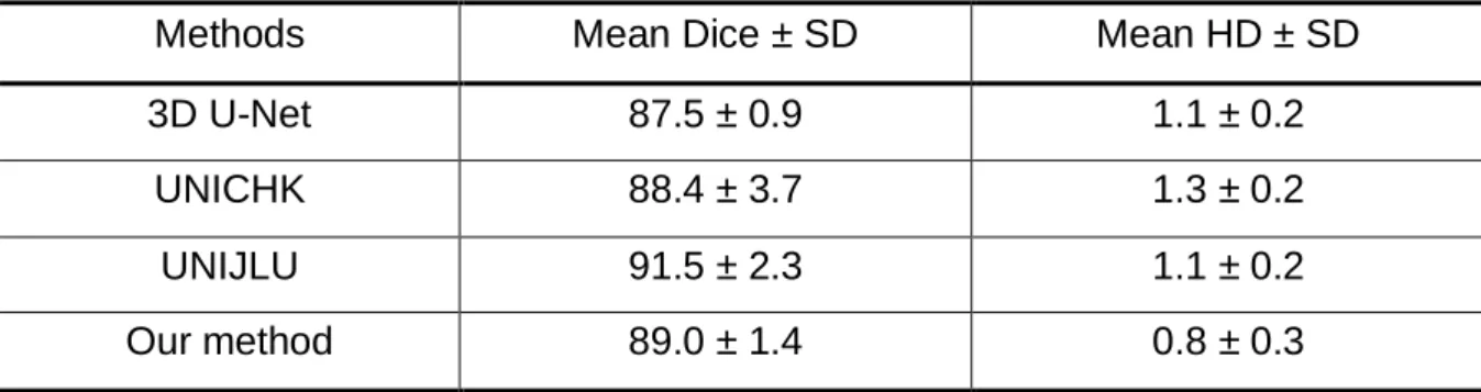
To evaluate the performance of the proposed methods, we compare the segmentation results achieved by our methods with those by 3D U-Net[15], the CNN-based team UNICHK [23] and the winning team UNIJLU [12] in the test1 dataset of the 2015 MICCAI Challenge [25]. Quantitative results evaluated with the different architectures are presented in Table 5. The mean Dice score obtained by our 3D method is 89.0% with a standard deviation (SD) of 1.4%. We bring a 1.5% boost comparing to the conventional 3D U-Net by training our network on 3D image patches extracted from opposed-phase, water, and fat images. This result is still 2.5% behind the state-of-the-art performance achieved by UNIJLU. The Mean HD of our 3D method reached 0.8 mm with an SD of 0.3 mm, which indicates that our method is slightly better when the segmentation results are reconstructed to 3D models. The strength of deep learning methods is the computation time. The Theano-based implementation of

Training dataset Combination Mean Dice ± SD

1) opp, wat, fat, and inn 87.9 ± 1.7

2) opp, wat, and fat 89.0 ± 1.4

3) opp, wat, and inn 88.0 ± 1.6

(34)

26

3D U-Net from UNICHK takes 3.1s to process one 40 × 512 × 512 volume. Our network is implemented based on TensorFlow and it takes about 0.5s to segment all the IVDs in a 36 × 256 × 256 input volume. Overall, the computation time of our end-to-end segmentation is about 10s including localization, preprocessing, segmentation and postprocessing. Whereas it takes 5 min on average to segment all IVDs for a patient by UNIJLU. It is also worth mentioning that the training dataset used in our study only contains data from 6 patients while UNICHK and UNIJLU have access to a training dataset from 16 patients i.e. our network is able to learn the 3D geometric morphometrics of IVDs with much fewer data to learn from.

Table 5. Segmentation result evaluation of the conventional 3D U-Net, UNICHK, UNIJLU and our method.

Methods Mean Dice ± SD Mean HD ± SD

3D U-Net 87.5 ± 0.9 1.1 ± 0.2

UNICHK 88.4 ± 3.7 1.3 ± 0.2

UNIJLU 91.5 ± 2.3 1.1 ± 0.2

Our method 89.0 ± 1.4 0.8 ± 0.3

Chapter 5: Conclusions

We attempted to solve two problems using deep learning: 1) the automated segmentation of chronic foot ulcers in a dataset we built on our own. 2) The automated segmentation of IVDs from 3D MRI scans. For evaluating the performance, we conducted comprehensive experiments and analyses on SegNet, VGG16, 2D U-Net, 3D U-Net and our model based on modified 3D U-Net and another proposed model based on MobileNetV2 and CCL. In the comparison of various neural networks, our

(35)

27

methods have demonstrated their effectiveness and in the field of medical image segmentation due to their fully convolutional architectures. We also demonstrated the robustness of our models by testing it on publicly available datasets where our model still achieves the highest Dice score. In the future, we plan to improve our work by extracting the shape features separately from the pixel-wise convolution in the deep learning model. Also, we will include more data in the dataset to improve the robustness and prediction accuracy of our method.

References

[1] Song, Bo, and Ahmet Sacan. Automated wound identification system based on image segmentation and artificial neural networks. In 2012 IEEE International Conference on Bioinformatics and Biomedicine. 1-4 (2012).

[2] A. I. Lopez, B. Glocker, “Complementary classification forests with graph-cut refinement for ivd localization and segmentation,” in Proc. the 3rd MICCAI Workshop & Challenge on Computational Methods and Clinical Applications for Spine Imaging, 2015.

[3] Fauzi, Mohammad Faizal Ahmad et al. Computerized segmentation and

measurement of chronic wound images. Computers in biology and medicine. 60, 74-85 (2015).

[4] D. Forsberg, "Atlas-based registration for accurate segmentation of thoracic and lumbar vertebrae in CT data," in Recent Advances in Computational Methods and Clinical Applications for Spine Imaging, pp. 49-59, Springer, Cham, 2015.

(36)

28

[5] C. Chen, D. Belavy, W. Yu, C. Chu, G. Armbrecht, M. Bansmann, D. Felsenberg, and G. Zheng, "Localization and segmentation of 3D intervertebral discs in MR images by data driven estimation," IEEE transactions on medical imaging, vol. 34, no. 8, pp. 1719-1729, 2015.

[6] Hettiarachchi, N. D. J., R. B. H. Mahindaratne, G. D. C. Mendis, H. T.

Nanayakkara, and Nuwan D. Nanayakkara. Mobile based wound measurement. In 2013 IEEE Point-of-Care Healthcare Technologies (PHT). 298-301 (2013). [7] Z. Wang, X. Zhen, K.Y. Tay, S. Osman, W. Romano, and S. Li. "Regression

segmentation for M3 spinal images," IEEE transactions on medical imaging, vol. 34, no. 8, 1640-1648, 2015.

[8] Hani, Ahmad Fadzil M., Leena Arshad, Aamir Saeed Malik, Adawiyah Jamil, and Felix Yap Boon Bin. Haemoglobin distribution in ulcers for healing assessment. In 2012 4th International Conference on Intelligent and Advanced Systems (ICIAS2012). 1, 362-367 (2012).

[9] Wantanajittikul, Kittichai, Sansanee Auephanwiriyakul, Nipon Theera-Umpon, and Taweethong Koanantakool. Automatic segmentation and degree

identification in burn colour images. In The 4th 2011 Biomedical Engineering International Conference. 169-173 (2012).

[10] H. Hutt, R. Everson, and J. Meakin, "3d intervertebral disc segmentation from MRI using supervoxel-based crfs," in International Workshop on Computational Methods and Clinical Applications for Spine Imaging, pp. 125-129, Springer,

(37)

29 Cham, 2015.

[11] M. Urschler, K. Hammernik, T. Ebner, and D. Štern, "Automatic intervertebral disc localization and segmentation in 3d mr images based on regression forests and active contours," In International Workshop on Computational Methods and Clinical Applications for Spine Imaging, pp. 130-140, Springer, Cham, 2015. [12] R. Korez, B. Ibragimov, B. Likar, F. Pernuš, and T. Vrtovec. "Deformable

model-based segmentation of intervertebral discs from MR spine images by using the SSC descriptor," in International Workshop on Computational Methods and Clinical Applications for Spine Imaging, pp. 117-124, Springer, Cham, 2015. [13] Krizhevsky, Alex, Ilya Sutskever, and Geoffrey E. Hinton. Imagenet classification

with deep convolutional neural networks. In Advances in neural information processing systems. 1097-1105 (2012).

[14] Russakovsky, Olga et al. Imagenet large scale visual recognition challenge. International journal of computer vision. 115, no. 3, 211-252 (2015).

[15] Garcia-Garcia, Alberto, Sergio Orts-Escolano, Sergiu Oprea, Victor Villena-Martinez, and Jose Garcia-Rodriguez. A review on deep learning techniques applied to semantic segmentation. arXiv preprint arXiv:1704.06857 (2017). [16] LeCun, Yann, Léon Bottou, Yoshua Bengio, and Patrick Haffner. Gradient-based

learning applied to document recognition. Proceedings of the IEEE. 86, no. 11, 2278-2324 (1998).

(38)

30

networks for semantic segmentation. In Proceedings of the IEEE conference on computer vision and pattern recognition. 3431-3440 (2015).

[18] Wang, Changhan et al. A unified framework for automatic wound segmentation and analysis with deep convolutional neural networks. In 2015 37th annual international conference of the IEEE engineering in medicine and biology society (EMBC). 2415-2418 (2015).

[19] Goyal, Manu, Moi Hoon Yap, Neil D. Reeves, Satyan Rajbhandari, and Jennifer Spragg. Fully convolutional networks for diabetic foot ulcer segmentation. In 2017 IEEE international conference on systems, man, and cybernetics (SMC). 618-623 (2017).

[20] Liu, Xiaohui et al. A framework of wound segmentation based on deep convolutional networks. In 2017 10th International Congress on Image and Signal Processing, BioMedical Engineering and Informatics (CISP-BMEI). 1-7 (2017).

[21] H. Chen, Q. Dou, X. Wang, J. Qin, J. CY Cheng, and P. A. Heng, "3D fully convolutional networks for intervertebral disc localization and segmentation," in International Conference on Medical Imaging and Virtual Reality, pp. 375-382, Springer, Cham, 2016.

[22] X. Li, Q. Dou, H. Chen, C. Fu, X. Qi, D. L. Belavý, G. Armbrecht, D. Felsenberg, G. Zheng, and P. A. Heng, "3D multi-scale FCN with random modality voxel dropout learning for Intervertebral Disc Localization and Segmentation from

(39)

31

Multi-modality MR Images," Medical image analysis, vol. 45, pp. 41-54, 2018. [23] H. Chen, Q. Dou, X. Wang, P. A. Heng, “Deepseg: Deep segmentation network

for intervertebral disc localization and segmentation,” in Proc. 3rd MICCAI Workshop & Challenge on Computational Methods and Clinical Applications for Spine Imaging, 2015.

[24] Ö. Çiçek, A. Abdulkadir, S. S. Lienkamp, T. Brox, and O. Ronneberger, "3D U-Net: learning dense volumetric segmentation from sparse annotation," in

International Conference on Medical Image Computing and Computer-Assisted Intervention, pp. 424-432. Springer, Cham, 2016.

[25] G. Zheng, C. Chu, D. L. Belavý, B. Ibragimov, R. Korez, T. Vrtovec, and H. Hutt et al, "Evaluation and comparison of 3D intervertebral disc localization and segmentation methods for 3D T2 MR data: A grand challenge," Medical image analysis, vol. 35, pp. 327-344, 2017.

[26] S. Kim, W. Bae, K. Masuda, C. Chung, and D. Hwang, "Fine-grain segmentation of the intervertebral discs from MR spine images using deep convolutional neural networks: BSU-Net," Applied Sciences, vol. 8, no. 9, pp. 1656, 2018.

[27] J. Dolz, C. Desrosiers, and I. B. Ayed, "IVD-Net: Intervertebral disc localization and segmentation in MRI with a multi-modal Unet," arXiv preprint

arXiv:1811.08305, 2018.

[28] J. T. Lu, S. Pedemonte, B. Bizzo, S. Doyle, K. P. Andriole, M. H. Michalski, R. G. Gonzalez, and S. R. Pomerantz. "DeepSPINE: Automated Lumbar Vertebral

(40)

32

Segmentation, Disc-level Designation, and Spinal Stenosis Grading Using Deep Learning," arXiv preprint arXiv:1807.10215, 2018.

[29] Sandler, Mark, Andrew Howard, Menglong Zhu, Andrey Zhmoginov, and Liang-Chieh Chen. Mobilenetv2: Inverted residuals and linear bottlenecks. In

Proceedings of the IEEE conference on computer vision and pattern recognition. 4510-4520 (2018).

[30] C. Chen, D. Belavy, and G. Zheng, "3D intervertebral disc localization and segmentation from MR images by data-driven regression and classification," in International Workshop on Machine Learning in Medical Imaging, pp. 50-58, 2014.

[31] Redmon, Joseph, and Ali Farhadi. Yolov3: An incremental improvement. Preprint at arXiv:1804.02767 (2018).

[32] Tzutalin. LabelImg. Git code https://github.com/tzutalin/labelImg (2015). [33] Chollet, François. Xception: Deep learning with depthwise separable

convolutions. In Proceedings of the IEEE conference on computer vision and pattern recognition. 1251-1258 (2017).

[34] Nair, Vinod, and Geoffrey E. Hinton. Rectified linear units improve restricted boltzmann machines. In Proceedings of the 27th international conference on machine learning (ICML-10). 807-814 (2010).

[35] Krizhevsky, Alex, and Geoff Hinton. Convolutional deep belief networks on cifar-10. Unpublished manuscript. 40, 1-9 (2010).

(41)

33

[36] Everingham et al. The pascal visual object classes challenge: A retrospective. International journal of computer vision. 111, no. 1, 98-136 (2015).

[37] Pearce, David J. An improved algorithm for finding the strongly connected components of a directed graph. Victoria University, Wellington, NZ, Tech. Rep (2005).

[38] S. Park, and N. Kwak, "Analysis on the dropout effect in convolutional neural networks," in Asian Conference on Computer Vision, pp. 189-204. Springer, Cham, 2016.

[39] Li, Fangzhao, Changjian Wang, Xiaohui Liu, Yuxing Peng, and Shiyao Jin. A composite model of wound segmentation based on traditional methods and deep neural networks. Computational intelligence and neuroscience. (2018).

[40] Zou, Kelly H. et al, Statistical validation of image segmentation quality based on a spatial overlap index1: scientific reports. Academic radiology. 11, no. 2, 178-189 (2004).

[41] F. Chollet et al, Keras, chollet2015keras, https://keras.io.

[42] S. S. Girija, Tensorflow: Large-scale machine learning on heterogeneous distributed systems. (2016).

[43] Kingma, Diederik P., and Jimmy Ba. Adam: A method for stochastic optimization. Preprint at arXiv:1412.6980 (2014).

[44] He, Kaiming, Xiangyu Zhang, Shaoqing Ren, and Jian Sun. Delving deep into rectifiers: Surpassing human-level performance on imagenet classification. In

(42)

34

Proceedings of the IEEE international conference on computer vision. 1026-1034 (2015).

[45] Ronneberger, Olaf, Philipp Fischer, and Thomas Brox. U-net: Convolutional networks for biomedical image segmentation. In International Conference on Medical image computing and computer-assisted intervention. 234-241 (2015). [46] Thomas, Stephen. Stock Pictures of Wounds. Medetec Wound Database

http://www.medetec.co.uk/files/medetec-image-databases.html (2020).

[47] Q. Fang, and D. A. Boas. "Tetrahedral mesh generation from volumetric binary and grayscale images," in Biomedical Imaging: From Nano to Macro, ISBI'09, IEEE International Symposium, pp. 1142-1145, 2009.