© 2011 R. Parimala, Dr. R. Nallaswamy. This is a research/review paper, distributed under the terms of the Creative Commons Attribution-Noncommercial 3.0 Unported License http://creativecommons.org/licenses/by-nc/3.0/), permitting all non-commercial
Volume 11 Issue 7 Version 1.0 May 2011
Type: Double Blind Peer Reviewed International Research Journal
Publisher: Global Journals Inc. (USA)
ISSN:
0975-4172
& Print ISSN:
0975-4350
A Study of Spam E-mail classification using Feature Selection
package
By R. Parimala, Dr. R. Nallaswamy
National Institute of Technology
Abstract-
Feature selection (FS) is the technique of selecting a subset of relevant features for
building learning models. FS algorithms typically fall into two categories: feature ranking and
subset selection. Feature ranking ranks the features by a metric and eliminates all features that
do not achieve an adequate score. Subset selection searches the set of possible features for the
optimal subset. Many FS algorithm have been proposed. This paper presents a new FS
technique which is guided by Fselector Package. The package Fselector implements a novel FS
algorithm which is devoted to the feature ranking and feature subset selection of high
dimensional data. This package provides functions for selecting attributes from a given dataset.
Attribute subset selection is the process of identifying and removing as much of the irrelevant
and redundant information as possible. The R package provides a convenient interface to the
algorithm. This paper investigates the effectiveness of twelve commonly used FS methods on
spam data set. One of the basic popular methods involves filter which select the subset of
feature as preprocessing step independent of chosen classifier, Support vector machine
classifier. The algorithm is designed as a wrapper around five classification algorithms. The
short description of the algorithm and performance measure of its classification is presented with
the spam data set.
Keywords:
GJCST Classification:
H.2.8, F.2.2
Strictly as per the compliance and regulations of:
A Study of Spam E-mail classification using Feature Selection package
A Study of Spam E-mail classification using
Feature Selection package
R. Parimala
α, Dr. R. Nallaswamy
ΩAbstract- Feature selection (FS) is the technique of selecting a subset of relevant features for building learning models. FS algorithms typically fall into two categories: feature ranking and subset selection. Feature ranking ranks the features by a metric and eliminates all features that do not achieve an adequate score. Subset selection searches the set of possible features for the optimal subset. Many FS algorithm have been proposed. This paper presents a new FS technique which is guided by Fselector Package. The package Fselector implements a novel FS algorithm which is devoted to the feature ranking and feature subset selection of high dimensional data. This package provides functions for selecting attributes from a given dataset. Attribute subset selection is the process of identifying and removing as much of the irrelevant and redundant information as possible. The R package provides a convenient interface to the algorithm. This paper investigates the effectiveness of twelve commonly used FS methods on spam data set. One of the basic popular methods involves filter which select the subset of feature as preprocessing step independent of chosen classifier, Support vector machine classifier. The algorithm is designed as a wrapper around five classification algorithms. The short description of the algorithm and performance measure of its classification is presented with the spam data set.
Keywords-FS, filter, wrapper, best-first search, SVM classification.
lassification is a method of categorizing or assi- -gning class labels to a pattern set under the sup- -ervision of teacher. It is one of the familiar and popular techniques in machine learning. The decisions boundaries are generated to discriminate between patterns belong to different classes. The patterns are initially partitioned into training set and testing set randomly and the classifier is trained on the former. The testing set is used to evaluate the generalized capability of the classifier. When a classification problem has to be solved, the common approach is to compute a wide variety of features that will carry as much as possible different information to perform the classification of samples. Thus, numerous features are used whereas, generally, only a few of them are relevant for the classification task, including the other in the feature set
Aboutα- R. Parimala, Assistant professor in Computer science
Department, Periyar E.V.R. College, Tiruchirapalli, India. (email: [email protected]).
About Ω- Dr. R. Nallaswamy, Profeesor, Department of Mathematics,
National Institute of Technology, Tiruchirapalli, India. (email:[email protected]).
used to represent the samples to classify, may lead to a slower execution of the classifier, less understandable results, and much reduced accuracy[1]. The irrelevant features are filtered out before the classification process[1]. Their main advantage is that their low computational complexity which makes them very fast. Their main drawback is that they are not optimized to be used with a particular classifier as they are completely independent of the classification stage.
Kira and Rendell (1992) described a statistical feature selection algorithm called RELIEF that uses instance based learning to assign a relevance weight to each feature [2][3]. John, Kohavi and Pfleger (1994) addressed the problem of irrelevant features and the subset selection problem. Further, they claim that the filter model approach to subset selection should be replaced with the wrapper model [4]. Koller and Sahami (1996) examined a method for feature subset selection based on Information Theory: they presented a theoretically justified model for optimal feature selection based on using cross-entropy to minimize the amount of predictive information lost during feature elimination [5]. Dash and Liu (1997) gave a survey of feature selection methods for classification. In a comparative study of feature selection methods in statistical learning of text categorization (with a focus is on aggressive dimensionality reduction)[34], Yang and Pedersen (1997) evaluated document frequency (DF), information gain (IG), mutual information (MI), a χ 2 test (CHI) and term strength (TS); and found IG and CHI to be the most effective[20]. Kohavi and John (1997) introduced wrappers for feature subset selection[4]. Their approach searches for an optimal feature subset tailored to a particular learning algorithm and a particular training set. Xing, Jordan and Karp (2001) successfully applied feature selection methods (using a hybrid of filter and wrapper approaches) to a classification problem.
Naïve Bayes Network algorithms were used frequently and they have shown a considerable success in filtering English spam e-mails [1]. Knowledge-based and rule-based systems were also used by researchers for English spam filters [2] [3]. As an alternative to these classical learning paradigms used frequently in spam filtering domain, evolutionary method was employed for classification and compared with Naïve Bayes
Global Journal of Computer Science and Technology Volume XI Issue VII Version I
20
11
45Ma
y
I.I
NTRODUCTIONC
classification [4]. It was argued that they show similar success rates although the former outperforms the Naïve Bayes classifier in terms of speed.
In this section, we discuss the basic concepts related to our research. Topics include a brief background on FS, methods, Feature Ranking and Feature subset Algorithms.
FS is frequently used as a preprocessing step to machine learning. It is a process of choosing a subset of original features so that the feature space is optimally reduced according to a certain evaluation criterion. FS has been a fertile field of research and development since 1970's and proven to be effective in removing irrelevant and redundant features, increasing efficiency in learning tasks, improving learning performance like predictive accuracy, and enhancing comprehensibility of learned results[4]. In recent years, data has become increasingly larger in both the number of instances and the number of features in many applications.
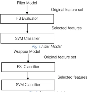
Techniques for FS can be divided in two approaches: feature ranking and subset selection. In the first approach, features are ranked by some criteria and then features above a defined threshold are selected. In the second approach, one searches a space of feature subsets for the optimal subset. Moreover, FS methods can broadly fall into two broad categories, the filter model or the wrapper model [2]. The filter model relies on general characteristics of the training data to select some features without involving any learning algorithm. The wrapper model requires one pre determined learning algorithm in FS and uses its performance to evaluate and determine which features are selected. As for each new subset of features, the wrapper model needs to learn a hypothesis (or a classifier). It tends to find features better suited to the predetermined learning algorithm resulting in a superior learning performance, but it also tends to be more computationally expensive than the filter model [5]. When the number of features becomes very large the filter model is usually chosen due to its computational efficiency.
Fig 1.Filter Model
Fig 2.Wrapper Model
In wrapper approaches learning algorithms are used to evaluate the quality of each feature. Specifically, a learning algorithm is run on a feature subset, and the classification accuracy of the feature subset is taken as a measure for feature quality. Generally, wrapper approaches are more computational demanding as compared with filter approaches. However, wrapper approaches often are superior in accuracy when compared with filters approaches which ignore the properties of the learning task in hand. In most application of SVM classification tasks, accuracy plays a greater role as compared with that of computational cost. Both approaches, filters and wrappers, usually involve combinatorial searches through the space of possible feature subsets. In the past few decades, researchers have developed large amount of FS algorithms. These algorithms are designed to serve different purposes, are of different models, and all have their own advantages and disadvantages. Various feature ranking and FS techniques have been proposed such as Correlation-based FS (CFS), Chi-square Feature Evaluation, Information Gain (IG), Gain Ratio (GR), Symmetric Uncertainty (SU), oneR and ReliefF. The feature ranking algorithms are implemented based on the code from Fselector package. The FSelector Package was created by Piotr Romanski and released in April 11, 2009.
The primary purpose of feature ranking approach is to reduce the dimensionality to decrease the computation time. This is particularly important concerning text categorization where the high dimensionality of the feature space is a problem. In many cases the number of features is in the tens of thousands. Then it is highly desirable to reduce this
FS Evaluator
SVM Classifier
Original feature set
Selected features
FS Classifier
SVM Classifier
Original feature set
Selected features WrapperModel
Global Journal of Computer Science and Technology Volume XI Issue VII Version I
20
11
46Ma
y
Filter Modelnumber, preferably without any loss in accuracy. Several FS methods have been proposed.
The general algorithm for the Feature Ranking Approach is:
for each feature Fi
wfi = getFeatureWeight(Fi) add wfi to wt_list
sort wt_list
choose top-k features.
a) Correlation based FS (CFS)
CFS evaluates the worth of a subset of attributes by considering the individual predictive ability of each feature along with the degree of redundancy between them. Yang & Pedersen, 1997 is used to measure the association between a class and features, as well as inter-correlations between the features. Relevance of a group of features grows with the correlation between features and classes, and decreases with growing inter-correlation[1]. CFS is used to determine the best feature subset and is usually combined with search strategies such as forward selection, backward elimination, bi-directional search, best-first search and genetic search. Among given features, it finds out an optimal subset which is best relevant to a class having no redundant feature. It evaluates merit of the feature subset on the basis of hypothesis--"Good feature subsets contain features highly correlated with the class, yet uncorrelated to each other [7]". This hypothesis gives rise to two definitions. One is feature class correlation and another is feature-feature correlation. Feature-class correlation indicates how much a feature is correlated to a specific class while feature-feature correlation is the correlation between two features. Equation 1, also known as Pearson‘s correlation, gives the merit of a feature subset consisting of k number of features. The CFS method is based on the ―merit‖ criterion.
Equation for CFS is given is equation
ii zi zc r k k k r k r 1 (1)where rzc is the correlation between the summed feature subsets and the class variable, k is the number of subset features,
zi
r is the average of the correlations between the subset features an the class variable, and
ii
r is the average inter-correlation between subset features[7]. In CFS features can be classified into three disjoint categories, namely, strongly relevant, weakly relevant and irrelevant features [4]. Strong relevance of a feature indicates that the feature is always necessary for an optimal subset; it cannot be removed without
affecting the original conditional class distribution. Weak relevance suggests that the feature is not always necessary but may become necessary for an optimal subset at certain conditions. Irrelevance indicates that the feature is not necessary at all.
b) CHI (χ 2 statistic)
Chi-Squared attribute selection is based on the Chi-Squared Statistic with respect to the target class. The algorithm finds weights of discrete attributes basing on a chi-squared test. The χ2 test is used in statistics to test the independence between two events [6].
c) EN (Entropy-based Ranking)
Linear correlation may not be able to capture correlations that are not linear. Therefore non-linear correlation measures often adopted for measurement. It is based on the information-theoretical concept of entropy, a measure of the uncertainty of a random variable.
d) IG (Information Gain)
Information gain [27], of a term measures the number of bits of information obtained for category prediction by the presence or absence of the term in a document. Information Gain is a method that selects attributes based on informational value gained by creating a branch on the attribute with respect to the class. Information theory indices are most frequently used for feature evaluation. A probabilistic model of a nominal valued feature Y can be formed by estimating the individual probabilities of the values yεY from the trained data. Entropy is a measure of uncertainty or unpredictability in a system. The entropy of Y is given by
P y
p
y
Y y Y H ( )log2 . If the observed value of
Y in the training data are partitioned according to the value of a second feature x, and the entropy of Y with respect to the partitions induced by x is less than the entropy of Y prior to partitioning, then there is a relationship between feature Y and x. The entropy of Y after observing x is
Y
x
p
x
P
y
x
p
y
H
Y y X x(
)
(
/
)
log
2/
. Information gain is given by
Y H(Y/x) H Gain
X
H(X/Y
)H
y H(x) H(x,Y) H Information gain is a symmetrical measure. The amount of information gained about y after observing x is equal to the amount of information gained about x after observing y.
Global Journal of Computer Science and Technology Volume XI Issue VII Version I
20
11
47Ma
y
A Study of Spam E-mail classification using Feature Selection package
e) Gain Ratio
Gain Ratio is a modification to information gain that takes into account the number and size of daughter nodes into which an attribute splits the dataset with respect to the class. This dampens the preference that the information gain method has for attributes with large numbers of possible values. [8]
) ( ) , ( ) ( X H X Y H X H Y H Ratio Gain . f) Mutual InformationThe MIFS (Mutual Information FS) algorithm uses a forward selection (Battiti, 1994). Mutual Information is a measure of general interdependence between random variables (i.e., features and type).We define the mutual information, I[X; Y ] ,
I[X; Y ] = H[X] - H[X/Y ] = H[Y ] = H[Y /X] = H[Y ] + H[X] - H[X; Y ] g) Symmetrical Uncertainty
Symmetrical Uncertainty is another method that was devised to compensate for information gain‘s bias towards features with more values. It capitalizes on the symmetrical property of information gain. The symmetrical uncertainty between features and the target concept can be used to evaluate the goodness of features for classification [10]
Symmetrical uncertainty =
X H Y H Gain 2 h) OneROneR could be viewed as an extremely powerful filter, reducing all datasets to one feature. OneR algorithms find weights of discrete attributes basing on very simple association rules involving only one attribute in condition part. The algorithm uses OneR classifier to find out the attributes‘ weights. For each attribute it creates a simple rule based only on that attribute and then calculates its error rate [11].
i) Relief
The RELIEF, one of the most used filter methods was introduced by Kira and Rendell [2] In the RELIEF, the relevance weight of each feature is estimated according to its ability to distinguish instances belonging to different classes. Thus, a good feature must assume similar values for instances in the same class and different values for instances in other classes. The algorithm finds weights of continuous and discrete attributes basing on a distance between instances. The relevance weights are set to be zero for each feature and then are estimated iteratively. In order to do that, an instance is chosen randomly from the training dataset. Then, the RELIEF searches for two
closest neighbors to such instance, one in the same class, called the Nearest Hit and the other in the opposite class called the Nearest Miss. The relevance weight of each feature is modified in each step according to the distance of the instance to its Nearest Hit and Nearest Miss. The relevance weights continue to be updated by repeating the above process using a random sample of n instances drawn from the training dataset. Filter methods are fast but lack of robustness against interactions among features and feature redundancy. In addition, it is not clear how to determine the cut-off point for rankings to select only truly important features and exclude noise. ReliefF uses a nearest neighbor implementation to maintain relevancy scores for each attribute. It defines a good discriminating attribute as the attribute that has the same value for other attributes in the same class and different from attribute values in different classes. [7][8][9] The Weka implementation repeatedly evaluates an attribute‘s worth by considering the value of its n nearest neighbors of same and different classes. [4] A family of algorithms called Relief [4] is based on the feature weighting, estimating how well the value of a given feature helps to distinguish between instances that are near to each other. One advantage of Relief is that it is sensitive to feature interactions and can detect higher than pair wise interactions.
Wrappers use a search algorithm to search through the space of possible features and evaluate each subset by running a model on the subset. Wrappers can be computationally expensive and have a risk of over fitting to the model. Wrapper methods search through the space of feature subsets and calculate the estimated accuracy of a single learning algorithm for each feature that can be added to or removed from the feature subset. The feature space can be searched with various strategies, e. g., forwards (i. e., by adding attributes to an initially empty set of attributes) or backwards (i. e., by starting with the full set and deleting attributes one at a time). Usually an exhaustive search is too expensive, and thus non-exhaustive, heuristic search techniques like genetic algorithms, greedy stepwise, best first or random search are often used (see, for details, Kohavi and John (1997)). For extracting the wrapper subsets we used wrapper subset evaluator in combination with the best first search method. Filters are similar to Wrappers in the search approach, but instead of evaluating against a model, a simpler filter is evaluated.
In the feature subset selection approach, one searches a space of feature subsets for the optimal subset. Such approach is present on the FSelector package by wrappers techniques (e.g. best-first search,
Global Journal of Computer Science and Technology Volume XI Issue VII Version I
20
11
48Ma
y
backward search, forward search, hill climbing search). Those techniques works by informing a function that takes a subset and generate an evaluation value for that subset. A search is performed in the subsets space until the best solution can be found.
a) Feature Subset Selection Algorithm
The feature subset algorithm conducts a search for a good subset using the induction algorithm itself as part of the evaluation function. The accuracy of the induced classifiers is estimated using accuracy estimation techniques [4]. The wrapper approach conducts a search in the space of possible parameters. Wrapper approaches use a specific machine learning algorithm/classifiers and utilize the corresponding classification performance to select features. A search requires a state space, an initial state, a termination condition, and a search engine [15]. Best-first search is a more robust method than hill-climbing. The idea is to select the most promising node we have generated so far that has not already been expanded. Best-first search usually terminates upon reaching the goal. b) Searching the Feature Subset Space
The purpose of FS is to decide which of the initial (possibly large number) of features to include in the final subset and which to ignore. If there are n possible features initially, then there are 2n possible subsets. The only way to find the best subset would be to try them all---this is clearly prohibitive for all but a small number of initial features.
Various heuristic search strategies such as hill climbing and Best First [Rich and Knight, 1991] are often applied to search the feature subset space in reasonable time. Two forms of hill climbing search and a Best First search were trialed with the feature selector described below; the Best First search was used in the final experiments as it gave better results in some cases. The Best First search starts with an empty set of features and generates all possible single feature expansions. The subset with the highest evaluation is chosen and is expanded in the same manner by adding single features. If expanding a subset results in no improvement, the search drops back to the next best unexpanded subset and continues from there. Given enough time a Best First search will explore the entire search space, so it is common to limit the number of subsets expanded that result in no improvement. The best subset found is returned when the search terminates[12]. The general algorithm for the Feature Subset Selection approach is:
S = all subsets for each subset s in S evaluate(s)
return (the best subset).
1) LDA
Linear discriminant analysis (LDA) and the related Fisher's linear discriminant are methods used in statistics and machine learning to find a linear combination of features which characterize or separate two or more classes of objects or events. The resulting combination may be used as a linear classifier or, more commonly, for dimensionality reduction before later classification. The LDA problem is formulated as follows . Let
x
n be a feature vector. We seek to find a transformationx
x
,
:
n
m withm
n
, such that in the transformed space, minimum loss of discrimination occurs. In practice,m
is much smaller thann
. A common form of optimality criteria to be maximized is the functionJ
tr
(
S
W1S
B)
. In classical LDA, the corresponding input-space within-class and between-class scatter matrix are defined by,t k k K k k B n S ( )( ) 1
t k k n k k n n n K k W x x S k ( )( ) 1 1
nk n k n k k n x 1 1
K k nk k N 1 1 The LDA is to maximize in some sense the ratio of between-class and within-class scatter matrices after transformation. This will enable to choose a transform that keeps the most discriminative information while reducing the dimension. Precisely, we want to maximize the objective function
t w t B
S
S
max
The columns of the optimum
are the relative generalized eigenvectors corresponding to the firstp
maximal magnitude eigenvalues of the equation
w BS
S
[13]. 2) Random ForestRandom forest (or RF) is an ensemble classifier that consists of many decision trees and outputs the class that is the mode of the class's output by individual trees. Random forests are often used when we have very large training datasets and a very large number of input variables (hundreds or even thousands of input variables). A random forest model is typically made up of tens or hundreds of decision trees. The algorithm for inducing a random forest was developed by Leo Breimanand Adele Cutler [14].
Global Journal of Computer Science and Technology Volume XI Issue VII Version I
20
11
49Ma
y
3) RPART
Recursive PARTitioning is a fundamental tool in data mining. Classification and regression trees [18] can be generated through the rpart package [19]. The rpart programs build classification or regression models of a very general structure using a two stage procedure; the resulting models can be represented as binary trees. The tree is built by the following process: first the single variable is found which best splits the data into two groups The data is separated, and then this process is applied separately to each sub-group and so recursively until the subgroups either reach a minimum size or until no improvement can be made.
4) NAÏVE BAYES
The Naïve Bayes (NB) classifier is the simplest in terms of its ease of implementation [20]. In terms of a classifier Bayes theorem (4) can be expressed as
) ( ) ( ) / ( / F P C P C F P F C P ,where F is a set of features and C are the target class. One argument [35] is that with the independence assumption the classifier would produce poor probabilities, but the ratio between them would be approximately the same as using conditional probabilities. Using the somewhat ‗Naive‘ independence assumption gave birth to its name Naive Bayesian classifier. Using the assumption for independence, according to (1), the joint probability for all n features can be obtained as a product of the total individual probabilities.
/
( / ) 1P f C C F P n i i
) ( ) / ( ) ( / 1 F P C f P C P F C P n i i
The denominator P(F) is the probability of observing the features in any message and can be expressed as
( / ) 1 1 k n i i m k PCk P f C F P
Inserting (8) into (7) the formula used by the Naive Bayesian Classifier is obtained
) / ( ) ( ) / ( ) ( / 1 1 1
m k n i i k K n i i C f P C P C f P C P F C P 5) SVMSVM [18][19] separates two classes with vectors that pass through training data points. The separation is measured as the distance between the support vectors and is called the margin. SVM have
shown promising results concerning text categorization problems in several studies [20]. A recent study [21] demonstrated that its performance was good with reference to the spam domain.
Support vector machine and its parameters
The algorithm about SVM is originally established by Vapnik (1998). Since 1990s SVM has been a promising tool for data classification. This introduction to Support Vector Machines (SVMs) is based on [26], [27], [28] and [29]. Support vector machine [22], [23] has gained prominence in the field of machine learning. Its basic idea is to map data into a high dimensional space and find a separating hyper plane with the maximal margin[22][23]. The solutions to classification sought by kernel based algorithm such as the SVM are linear functions in feature space:
f(x)
w
T
x
for some weight vector w
F
.Given a training set of instance-label pairs
x y
i,
i
, i =1, 2, 3…ℓ, wherex R
i
n . The class label of the ith pattern is denoted by{1, 1}
ti
y
. Nonlinearly separable problem are often solved by mapping the input data samplesx
i to a higher dimensional feature space
x
i . The classical maximum margin SVM classifier aims to find a hyper plane of the form
0
t
w x b
that separates patterns of the two classes[30]. So far we have restricted ourselves to the case where the two classes are noise-free. In the case of noisy data, forcing zero training error will lead to poor generalization. To take account of the fact that some data points may be misclassified we introduce a vector of slack variables
(
1,
,
l)
T that measure the amount of violation of the constraints. The problem can then be written as , , 11
2
n t i w b iMinimize w w C
(2) Subject to the constraints
1
0,
1,2,3... ,
t i i i iy w
x
b
i
(3) The solution to (2)-(3) yields the soft margin classifier, so termed because the distance or margin between the separating hyper planew
t
x b
0
is usually determined by considering the dual problem, which is given by
T i i i i i i 2 γ ξ 1 b x φ w y α 2 w (4)where
( , , )
1
l T, as before, and are the Lagrange multipliersGlobal Journal of Computer Science and Technology Volume XI Issue VII Version I
20
11
50Ma
y
L w b a
( , , , ,
i
)
i=1 i=1 T l)
,
,
(
1
corresponding to the positivity of the slack variables. The solution of this problem is the saddle point of the Lagrangian given by minimizing
L
with respect to w,and
b
, and maximizing with respect to
0
and0
. Differentiating with respect tow
,b
and and setting the results equal to zero.We obtain 1 ( , , , , ) l ( ) 0 i i i L b y
w w x w 1 ( , , , , ) l 0 i i i L b y b w
, d ( , , , , ) 0. i i i L b C w (4)
1
1 1 1 1 , 2 i j i j i j i i j i Minimize y y k x x
to 0
Idi and 0i C i, 1,2,3... Here,
ii
1,2,3,....
denotes the.
Lagrange multipliers and the matrix
i, j
i .
jK x x
x
x are termed as Kernel matrix. Kernel based learning methods use an implicit mapping of the input data into a high dimensional feature space defined by a kernel function. Training vectorx
i is mapped into a higher dimensional feature space and then the learning takes place in the feature space [24][25]. In this paper, we focus our attention to the RBF kernels: K x x
i, j
xi .
xj .Package kernlab [27, 28] aims to provide the R user with basic kernel functionality (e.g., like computing a kernel matrix using a particular kernel), along with some utility functions commonly used in kernel-based methods like a quadratic programming solver, and modern kernel-based algorithms based on the functionality that the package provides.
ksvm() in kernlab package [27, 28] is a flexible SVM implementation which includes the most SVM formulations and kernels and allows for user defined kernels as well. It provides many useful options and features like a method for plotting, class probabilities output, cross validation error estimation.
a) K-Fold Cross Validation
When we have finished the FS, we use the SVM to do the classification. The cross validation will help to identify good parameters so that the classifier can
accurately predict unknown data. In this paper, we used 10 fold cross validation to choose the penalty parameter C and γ in the SVM. When we get the nice arguments, we will use them to train model and do the final prediction [33].
b) Used Environment and Libraries
There are several libraries available for FS and SVMs. Fselector package provides functions for selecting attributes from a given dataset. Attribute subset selection is the process of identifying and removing as much of the irrelevant and redundant information as possible. This package contains Algorithms for filtering attributes, Algorithms for wrapping classifiers and search attribute subset space such as best first search, backward search, forward search and hill climbing search and Algorithm for choosing a subset of attributes based on attributes‘ weights.
The environment used in this work is R [30] together with the package kernlab [27][28]. Kernlab is a package that offers several methods for kernel-based learning. The program was written in R programming language. The PC we used for experiment has the machine used was an Intel Core 2 Duo E7500 @ 2.93GHz with 2GB RAM.
c) Datasets and Data Preprocessing
The data of the spam email problem in this paper is downloaded from the UCI Machine Learning Repository [31][32]. There are a total of 4601 emails in the database, i.e., the training set is of size 4601, 1813 of which are labeled as spam, the rest as non-spam. In addition to this class label there are 57 variables indicating the frequency of certain words and characters in the e-mail. The first 48 variables contain the frequency of the variable name (e.g., business) in the e-mail. If the variable name starts with num (e.g., num650) it indicates the frequency of the corresponding number (e.g., 650). These words were deemed to be relevant for distinguishing between spam and non-spam emails. They are as follows: make, address, all, 3d, our, over, remove, internet, order, mail, receive, will, people, report, addresses, free, business, email, you, credit, your, font, 000, money, hp, hpl, george, 650, lab, labs, 857, data, 415, 85, technology, 1999, parts, pm, direct, cs, meeting, original, project, re, edu, table, and conference. The variables 49-54 indicate the frequency of the characters ‗;‘, ‗(‘, ‗[‘, ‗!‘, ‗$‘, and ‗#‘. The variables 55-57 contain the average; longest and total run-length of capital letters. Variable 58 indicates the type of the mail and is either "non-spam" or "spam", i.e. unsolicited commercial e-mail. . Given an email text and a particular WORD, we calculate its frequency, i.e., the percentage of words in the e-mail that match WORD: word freq WORD =100 × r/t, where r is number of times the
Global Journal of Computer Science and Technology Volume XI Issue VII Version I
20
11
51Ma
y
A Study of Spam E-mail classification using Feature Selection package
= = 1 I= i = = = = =
WORD appears in the email and t is the total number of words in e-mail.
In order to obtain an averaged unbiased accuracy estimate, we conducted 25 runs. For each run, data are completely randomized, then the database is divided into a training set and a separate test set. d) Measuring the performance
The meaning of a good classifier can vary depending on the domain in which it is used. For example, in spam classification it is very important not to classify legitimate messages as spam as it can lead to e.g. economic or emotional suffering for the user. Classifiers have long been evaluated on their accuracy only. An often-used measure in the information retrieval and natural language processing communities is Overall Accuracy (OA). This is the most common and simplest measure to evaluate a classifier. It is just defined as the degree of right predictions of a model. Kappa statistic: (Kappa). This is originally a measure of agreement between two classifiers (Cohen, 1960), although it can also be employed as a classifier performance measure. This is the overall Accuracy corrected for agreement by chance. The kappa-statistic as proposed by Cohen (1960) is a coefficient to evaluate the agreement among several raters. We have the observations of two raters and assume that both raters classify statistically independent. The first mention of a kappa-like statistic is attributed to Galton (1892), see Smeeton (1985).
The equation for κ is:
In broad terms a kappa below 0.2 indicates poor agreement and a kappa above 0.8 indicates very good agreement beyond chance. Given a set of n elements S
O1,O2,....,On
and two partitions of S to compare, X
x1,x2,....,xr
andY
y1,y2,....,ys
, The Rand index, R, is:.
Intuitively, a + b can be considered as the number of agreements between X and Y and c + d as the number of disagreements between X and Y. The crand index is the Rand index corrected for agreement by chance. Fig.3, Fig.4 and Table1 shows the various performance measures.
Fig.3. Averaged Performance measures of various Feature Ranking methods.
Fig.4. Averaged Classification accuracy of various Filter and Wrapper methods.
Methods Feature % Accuracy
SVM 100 93.27 CFS-SVM 16 91.44 Chi-SVM 70 93.00 IG-SVM 70 93.00 GR-SVM 70 93.39 SU-SVM 70 93.33 oneR-SVM 70 92.65 Relief-SVM 70 93.15 Lda-SVM 32 91.90 Rpart-SVM 12 90.51 SVM-SVM 16 89.95 RF-SVM 21 91.23 NB-SVM 7 80.00
Table1: A comparison of Feature Percent and Accuracy
In this paper, we experiment several FS strategies to work on the spam e-mail data set. On the whole, the strategies with RBF kernel are better than the ones without it. In our evaluation, we test how the implemented FS can affect (i.e. improve) the accuracy of Support vector machine classifiers by performing FS. The results show that filter method CFS, Chi-squared, GR, ReliefF, SU, IG, oneR, enabled the classifiers to achieve the highest increase in classification accuracy on the average while reducing the number of unnecessary attributes. The primary purpose of FS is to
0.6 0.650.750.80.7 0.850.9 0.951 Or igina l CF S Ch i-… IG GR SU on eR Re lief
Performance Measure of
various Feature Ranking
…
Accuracy Kappa Crand Rand
Global Journal of Computer Science and Technology Volume XI Issue VII Version I
20
11
52Ma
y
reduce the dimensionality to decrease the computation time. This is particularly important concerning text categorization where the high dimensionality of the feature space is a problem. In many cases the number of features is in the tens of thousands. Then it is highly desirable to reduce this number, preferably without any loss in accuracy. The reason for using these five FS methods CFS, LDA, RF, Rpart and NB among twelve FS methods in this study is that they all have shown good performance.
The experiments have shown that in many cases CFS gives results that are comparable or better than the wrapper, Because CFS make use of all the training data at once. The number of features selected by the wrapper using CFS is very Less is very faster than the wrapper, by more than an order of magnitude, which allows it to be applied to large size of the datasets than the wrapper.
The authors thank many people who have contributed to the R Package; in particular, acknowledgement to all contributors, R statistics, tools and code for their invaluable efforts.
1. Hall, M. A., Smith, L. A., 1997, Feature Subset Selection: A Correlation Based Filter Approach, International Conference on Neural Information Processing and Intelligent Information Systems, Springer, p855-858.
2. Kira, K., and Rendell, L. A. The feature selection problem: Traditional methods and a new algorithm. In Proceedings of the AAAI-92 (1992), AAAI Press, pp. 129-134.
3. Kira, K., and Rendell, L. A. A practical approach to feature selection. In The 9th International Conference on Machine Learning (1992), Morgan Kaufmann, pp. 249-256.
4. John, G. H., Kohavi, R., and Pflegger, K. Irrelevant features and the subset selection problem. In Machine learning: Proceedings of the Eleventh International Conference (1994), Morgan Kaufmann, pp. 121-129.
5. Sahami, M., Dumais S., Heckerman D., and Horvitz, E. (1998), A Bayesian approach to filtering junk e-mail. Learning for Text Categorization, Papers from the AAAI Workshop, Madison Wisconsin, pp. 55–62. AAAI Technical Report WS-98-05.
6. A.M. Mesleh, CHI Square Feature Extraction Based SVMs Arabic Language Text Categorization System, Proceedings of the 2nd International Conference on Software and Data Technologies, (Knowledge Engineering), Vol. 1,
Barcelona, Spain, July, 22—25, 2007, pp. 235-240.
7. Ghiselli E.E. Theory of Psychological Measure_ment, McGraw_Hill.
8. J.R. Quinlan, Induction of decision trees, Machine Learning 1, 81-106, 1986.
9. Battiti, R. (1994). Using mutual information for selecting features in supervised neural net learning. IEEE Trans. Neural Networks, 5(4):537–550.
10. Press, W. H., Flannery, B. P., Teukolsky, S. A., &Vetterling, W. T. (1988). Numerical recipes in C Cambridge University Press, Cambridge. 11. Holte, R.C. (1993) ―Very simple classification
rules perform well on most commonly used datasets.‖ Machine Learning, Vol. 11, 63–91. 12. Ginsberg, M. L 1993, Essentials of Artificial
Intelligence, Morgan Kaufmann.
13. Duchene and S. Leclercq, "An Optimal Transformation for Discriminant Principal Component Analysis," IEEE Trans. On Pattern Analysis and Machine Intelligence, Vol. 10, No 6, November 1988.
14. Breiman, L., 1998, ―Arcing classifiers. Annals of Statistics, 26(3):801– 849‖.
15. Breiman, L., Friedman, J. H., Olshen, R. A., and Stone, C. J. 1984, Classification and Regression Trees. Wadsworth International, Belmont, Ca.
16. Therneau TM, Atkinson EJ (1997). \An Introduction to Recursive Partitioning Using the rpart Routine." Technical Report 61, Section of Biostatistics, Mayo Clinic, Rochester,URL http://www.mayo.edu/hsr/techrpt/61.pdf. 17. I. Rish, An empirical study of the naive Bayes
classifier, IJCAI 2001, Workshop on Empirical Methods in Artificial Intelligence.
18. Vapnik V N., 1995, The nature of statistical learning theory. New York, Springer. 19. Vladimir N. Vapnik, The Nature of Statistical
Learning Theory. New York: Springer-Verlag, 1995, 187 pp.
20. Yang, Y., Pedersen, J.O., A Comparative Study on Feature Selection in Text Categorization, Proc. of the 14th International Conference on Machine Learning ICML97, pp. 412---420, 1997. 21. Androutsopoulos, I., Koutsias, J.: An Evaluation of Naive Bayesian Networks. In:Machine Learning in the New Information Age. Barcelona Spain (2000) 9-17.
Cristianini, N., and Shawe-Taylor, J., 2000, ―An introduction to support vector machines. Cambridge, UK: Cambridge University Press‖. 23. Cristianini, N., and Shawe-Taylor, J., 2003‖.
Support Vector and Kernel Methods,
Global Journal of Computer Science and Technology Volume XI Issue VII Version I
20
11
53Ma
y
A Study of Spam E-mail classification using Feature Selection package
22.
References Références Referencias
Intelligent Data Analysis: An Introduction Springer – Verlag‖.
Schölkopf, B., Burges, C.J.C., and Smola, A.J., (Eds.), 1998,‖ Advances in Kernel Methods: Support Vector Learning, MIT Press.
25. Smola, A.J., and Scholkopf, B., Learning with kernels: Support Vector Machines, regularization, optimization, and beyond, Cambridge, MA: MIT press‖.
26. Burges, C.J.C., 1998,‖ A tutorial on support vector machines for pattern recognition. Data Mining and Knowledge Discovery, 2(2):121–167‖.
27. Karatzoglou , A., Smola, A., Hornik, K,, Zeileis,A.,2005,―kernlab – Kernel Methods.‖ R package, Version 0.6-2. Available from http://cran.R-project.org.
28. Karatzoglou, A., Smola, A., Hornik, K., Zeileis, A., 2004, ― kernlab – An S4 Package for Kernel Methods in R.‖ Journal of Statistical Software,11(9). URL http://www.jstatsoft.org/v11/io9/‖.
29. Chih-Chung Chang., Chih-Jen Lin.,, 2001, ―Libsvm: a library forsupport vector machines.http://www.csie.ntu.edu.tw/˜cjlin/libsv m‖.
30. R Development Core Team (2009). R: A Language and Environment for Statistical Computing. R Foundation for Statistical Computing, Vienna, Austria. ISBN 3-900051-07-0,URLhttp://www.R-project.org/.
31. Leisch,F.,Dimitriadou,E.,2001,―mlbench—A Collection for Artificial and Real-world Machine Learning Benchmarking Problems.‖R package, version 0.5-6. Available from http://CRAN.R-project.org.
32. Hettich, S., Blake, C. L., and Merz, C. J., 1998,‖ UCI repository of Machine learning databases, Department of Information and Computer Science, University of California, Irvine, CA‖,.http://www.ics.uci.edu/~mlearn/ MLRepository.html‖
33. Dimitriadou E, Hornik K, Leisch F, Meyer D, Weingessel A (2005), e1071: Misc Functions of the Department of Statistics (e1071), TU Wien, Version 1.5-11, URL http://CRAN.R-project.org/.
Dash, M., and Liu, H., 1997, Feature selection for classification. Intelligent Data Analysis: An International Journal‖, Vol. 1(3), pp. 131- 156. 35. Domingos, P., & Pazzani, M. (1996). Beyond
Independence: Conditions for the Optimality of the Simple Bayesian Classifier, Proceedings of the International Conference on Machine Learning.