UCLA
UCLA Electronic Theses and Dissertations
TitleInterpreting Nonlinear Black-box Models Globally: A Comparative Study of Different Techniques Permalink https://escholarship.org/uc/item/0t24x7xg Author Li, Yingqi Publication Date 2020 Peer reviewed|Thesis/dissertation
UNIVERSITY OF CALIFORNIA Los Angeles
Interpreting Nonlinear Black-box Models Globally: A Comparative Study of Different Techniques
A thesis submitted in partial satisfaction of the requirements for the degree
Master of Science in Statistics
by
Yingqi Li
c
Copyright by Yingqi Li
ABSTRACT OF THE THESIS
Interpreting Nonlinear Black-box Models Globally: A Comparative Study of Different Techniques
by Yingqi Li
Master of Science in Statistics University of California, Los Angeles, 2020
Professor Jingyi Li, Chair
In machine learning, black-box models that discover underlying relationships in data are more predictive than white-box models, but also more challenging to interpret. The con-straint of interpretability for nonlinear black-box models is rooted in the interaction effects between features. Based on modeling needs, a white-box model may be sufficient in some circumstances, but understanding how a black-box model generates predictions is essen-tial out of consideration for accuracy and faithfulness. In this paper, we use three global, model-agnostic interpretability methods (Partial Dependence Plot and Individual Condi-tional Expectation Plot, Global Surrogate, and Global SHAP through discretization) to explain a diverse class of black-box models and compare their behavior quantitatively and qualitatively. The experiment results demonstrate that the performance of the methods varies when the datasets and black-box models in need of interpretation are different. We prove that the methods provide explanations from several perspectives, and therefore present a strategy that selects the most appropriate interpretability method given a new model on a new dataset.
The thesis of Yingqi Li is approved.
Hongquan Xu Chad J Hazlett Jingyi Li, Committee Chair
University of California, Los Angeles 2020
To my mother and father,
who encouraged me to set goals and accomplish them through small daily improvement
TABLE OF CONTENTS
1 Introduction . . . 1
2 Interpretability . . . 3
2.1 White-box vs. Black-box Models . . . 3
2.2 Being Global and Model-agnostic . . . 5
2.3 Evaluating Interpretability Methods . . . 6
3 Experiments . . . 8
3.1 Methods and Datasets . . . 8
3.1.1 PD Plot and ICE Plot . . . 9
3.1.2 Global Surrogate . . . 11
3.1.3 Global SHAP . . . 11
3.2 Analyzing Feature Correlations . . . 13
4 Explaining Wine Quality Predictions . . . 14
4.1 PD Plot and ICE Plot Explanations . . . 15
4.2 Global Surrogate Explanations . . . 20
4.3 Global SHAP Explanations . . . 24
5 Explaining Credit Predictions. . . 30
5.1 PD Plot and ICE Plot Explanations . . . 31
5.2 Global Surrogate Explanations . . . 36
5.3 Global SHAP Explanations . . . 39
6.1 Advantages and Disadvantages . . . 42
6.2 Towards a Selection Strategy . . . 43
6.3 Further Discussions . . . 45
6.3.1 Faithfulness of Explanations . . . 46
6.3.2 Interpretability on Image Data and Neural Networks . . . 46
LIST OF FIGURES
4.1 PD plot and ICE plot for alcohol and sulphates by RF on the wine quality data. The y-axis represents Pr(quality = good). The yellow line is PD plot. Each blue line represents the ICE plot of a cluster of instances, with 20 clusters in total. Each blue bin displays the percentage of instances whose feature value falls into the range. . . 16 4.2 PD plot and ICE plot for alcohol and sulphates by SVM on the wine quality data
after standardization . . . 17 4.3 PD plot and ICE plot for alcohol and sulphates by GBM on the wine quality data 18 4.4 PD plot and ICE plot for alcohol and sulphates by NN on the wine quality data
after standardization . . . 19 4.5 Surrogate tree model for RF on the wine quality data. Surrogate tree model for
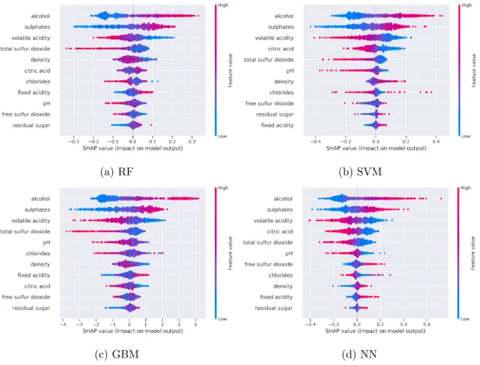
GBM is the same. . . 21 4.6 Surrogate tree model for SVM on the wine quality data after standardization . . 22 4.7 Surrogate tree model for NN on the wine quality data after standardization . . . 23 4.8 SHAP summary plot for RF, SVM, GBM, and NN on the wine quality data.
Each point represents an instance. Being red means having a high feature value. Features are ranked by the total magnitude of SHAP values on all instances in descending order. The x-axis states the magnitude of effects and the direction of effects for each instance. . . 25 4.9 SHAP dependence plot for RF on the wine quality data. Each point represents an
instance, and each plot is the dependence plot of the feature on the x-axis when using SHAP values. The right y-axis states the feature that correlates with the feature on the x-axis most. Being red means having a high value in the feature on the right y-axis. . . 26 4.10 SHAP dependence plot for SVM on the wine quality data after standardization 27
4.11 SHAP dependence plot for GBM on the wine quality data . . . 28
4.12 SHAP dependence plot for NN on the wine quality data after standardization . 29 5.1 PD plot and ICE plot for ExternalRiskEstimate and NetFractionRevolvingBur-den by RF on the credit data. The y-axis represents Pr(RiskPerformance = Bad). 32 5.2 PD plot and ICE plot for ExternalRiskEstimate and NetFractionRevolvingBur-den by SVM on the credit data after standardization . . . 33
5.3 PD plot and ICE plot for ExternalRiskEstimate and NetFractionRevolvingBur-den by XGB on the credit data . . . 34
5.4 PD plot and ICE plot for ExternalRiskEstimate and NetFractionRevolvingBur-den by NN on the credit data after standardization . . . 35
5.5 Surrogate tree model for RF on the credit data . . . 37
5.6 Surrogate tree model for SVM on the credit data after standardization . . . 37
5.7 Surrogate tree model for XGB on the credit data . . . 38
5.8 Surrogate tree model for NN on the credit data after standardization . . . 38
5.9 SHAP summary plot for RF, SVM, XGB, and NN on the credit data . . . 40
5.10 SHAP dependence plot of the three most important features for RF, SVM, XGB, and NN on the credit data . . . 41
LIST OF TABLES
3.1 Data summary and model performance evaluated by F1 scores, AU-ROC values, and AU-PRC values. Default means failure to repay a loan. . . 9
4.1 Global accuracy and fidelity (both measured with F1 score) of the explanation models in predicting good-quality red wine . . . 14
5.1 Global accuracy and fidelity (both measured with F1 score) of the explanation models in predicting loan default . . . 30
ACKNOWLEDGMENTS
I would like to express my great gratitude to Professor Jingyi Li, my thesis advisor, for offering me time to discuss the topic from the very start and guidance of solving the obstacles I encountered during the entire research process. Her enthusiasm and expertise in Statistics have influenced me deeply during my master’s study. I am also grateful for the constructive suggestions given by Professor Hongquan Xu and Professor Chad J Hazlett, who directed me towards a better thesis with extensive knowledge and patience.
I would also like to particularly thank Loek Janssen, my internship supervisor, for his engagement, constant support, and insightful advice in steering me in the path of useful research that is applicable in practice. My sincere thanks are also extended to Sarah Davies at Nova Credit, who leads me to the field of credit scoring where the thesis topic originated.
CHAPTER 1
Introduction
Machine learning has become a useful tool for solving real-world problems, e.g., establishing a spam filter, building recommendation systems for online shopping, and detecting fraud in real-time. These cases usually have complex data that cannot be handled by simple models; therefore, a black-box model that uncovers underlying relationships between features is needed. The improvement in accuracy comes with a decrease in interpretability for black-box models. People see the predictions but cannot understand how the predictions are generated or what are the critical features that lead to the results.
An understanding of how a model makes decisions is essential, and researchers may sac-rifice accuracy for a simpler but more explainable model in some cases. For example, in credit scoring, a data scientist may choose a logistic regression model over a neural network with more accurate predictions. It is because logistic regression shows feature importance explicitly and states the reason why loan applications are denied, e.g., excessive inquiries or high credit utilization rate. To overcome such a tradeoff between accuracy and interpretabil-ity, we explain how black-box models function globally using three post hoc interpretability methods. My contributions are:
• An extensive number of tests on global interpretability methods for comparison
• A discretization method for aggregating local feature attributions towards a global explanation model
• A combination of quantitative measurement and qualitative evaluation of explanations, providing a consistency examination on the magnitude, direction, and shape of feature effects and the interaction between features
• A comprehensive strategy for choosing the most appropriate interpretability method given a new black-box model on a new dataset
CHAPTER 2
Interpretability
The notion of interpretability describes the ability of a model to explain the relationships be-tween input and output [RSG16, DK17], i.e., how a model predicts from the input features. It plays an essential role in choosing from models [RSG16], notably when black-box models, which are hard to interpret [Fre14], outperform those straightforward ones. Although ma-chine learning practitioners often use accuracy to measure model performance quantitatively, choosing the best model based solely on accuracy may lead to biased decisions due to data leakage [RSG16]. It means that the training data contains some information that will not show in the testing data, and the additional information could cause accuracy no longer to be accurate. Complete reliance on predictive power without knowing what is going on be-hind the scene may also lead to potential danger. According to Adadi and Berrada [AB18], in the 1990s, researchers abandoned a well-performed neural network trained to select the pneumonia patients needing treatment in the hospital, because they found the model was misleading after interpreting it. Therefore, a combination of accuracy and interpretation in evaluating model performance is necessary not only for trustworthiness but also for the sake of preventing severe consequences caused by incorrect decisions.
2.1
White-box vs. Black-box Models
When a white-box model, which explains itself, completes a modeling task with satisfactory results, there is no need to use a black-box model instead and then explain it with the assistance of external interpretability methods. In certain circumstances, a white-box model can become black-box like (e.g., a deeply nested tree model), and vice versa. Therefore,
before we investigate some interpretability methods, we clarify the boundary between white-box models and black-white-box models first.
The interpretability constraint on nonlinear black-box models is rooted in the interaction effects between features. We discuss how the interaction effects exist in some classic black-box models. (1) For tree ensemble models, e.g., random forest and gradient boosting machine, the interaction effects arise from the connection between tree nodes in different depths. A value change in the parent node can lead to a different path going down to the bottom of a tree. One will not know what the model output is unless following the path of each tree and aggregating the results of base learners. (2) For kernel support vector machine, the interaction effects arise from the kernel trick K(xi,xj) = φ(xi)>φ(xj), which projects data points from the raw feature space to a higher-dimensional space. Although projected data points in the high-dimensional space are linearly separable, the weights w=
P
iαiyiφ(xi) no longer stand for feature importance for the raw features but the transformed features, which are hard to interpret. (3) For deep neural networks, the interaction effects arise from the activation function and the hidden layers where hierarchical concepts are built on top of the neurons from previous layers.
Transformation between white-box and black-box models is possible. Classic lin-ear models, decision trees, and rule-based systems are examples of white-box models. These interpretable models often have stringent assumptions in terms of independence, distribu-tion, and variance. Some generalizations of these models loosen the assumptions and are also intrinsically explainable, e.g., generalized linear model (GLM), logistic regression with L1 regularization, and explainable boosting machine (EBM) [NJK19]. Some, on the contrary, become more like black-box models. One example is a tree model with deep and complex decision paths. Second, a black-box model that is not globally interpretable can change to a locally interpretable one. For example, a gradient boosting machine can preserve monotonic relationships between features and labels with enforced constraints [HG18]. It asserts that when we explain local instances, an increase in one feature will always have either positive
or negative effects on the prediction.
Use white-box models as baselines. There are circumstances when using a white-box model is enough for solving problems. Hall and Gill [HG18] propose the idea of establishing suitable white-box models based on decision functions related to linearity and monotonicity. For example, in credit scoring, when one has complex data but needs to comply with industry regulations, a monotonic GBM with nonlinear but monotonic function is better than a neural network with nonlinear and non-monotonic function [HG18]. When the baseline models fail, it is time to train a black-box model and provide explanations with some interpretability methods.
2.2
Being Global and Model-agnostic
There are two types of interpretability: (1) local interpretability, which means given an in-stance we can interpret how to obtain a single prediction, and (2) global interpretability, which means given a model we can inspect how the features work together towards the pre-dictions [AB18, Mol19]. There has been abundant research on local interpretability methods, including the controversial topic of the stability of local explanations [AJ18, MJ18]. In this paper, we concentrate on establishing global explanations for nonlinear black-box models, which decipher the most important features, their effect directions, and the interaction effects between them.
Global interpretability methods can be both model-specific and model-agnostic [RSG16, AB18, Mol19]. Model-specific methods apply to particular model types. To investigate methods with some flexibility in the model we choose, we will study model-agnostic inter-pretability methods in the following text.
2.3
Evaluating Interpretability Methods
To compare different interpretability methods, we view their explanation of a black-box model also as a model, which is proposed by Lundberg and Lee [LL17]. This perspective paves the way for quantitative measurement of their performance. Using the measurement approach adopted by Tan et al. [TCH18], we evaluate the performance of the explanation models with global accuracy and global fidelity (also used in [RSG16, LL17, GMR18]).
• Global accuracy: an evaluation metric that describes how accurately an explanation model predicts the true labels. To illustrate it more formally, supposeXn×p is a matrix with each row representing an instance and each column representing a feature, and
yn×1 is a vector representing the true labels to predict. ˆyn×1 stands for the predicted
labels of a black-box model. We takeXn×p as input and ˆyn×1 as the target to establish
a new explanation model, and ˆyn∗×1 stands for the predicted labels of the explanation model. LetL(·,·) be the loss function of a model; then global accuracy can be denoted as:
global accuracy =−L(ˆy∗,y). (2.1) Some examples of loss L are:
– Mean square error (MSE) for regression:
L(ˆy∗,y) = n X i=1 (yi−yˆi∗) 2/n (2.2)
– Mean absolute error (MAE) for regression:
L(ˆy∗,y) = n
X
i=1
|yi−yˆi∗|/n (2.3)
– Hinge loss for classification:
L(ˆy∗,y) = n
X
i=1
– Logistic loss for classification: L(ˆy∗,y) = n X i=1 −yilog(ˆy∗i)−(1−yi)log(1−yˆ∗i) (2.5)
• Global fidelity: an evaluation metric that describes how accurately an explanation model estimates the predicted labels of a black-box model, i.e., how precisely an ex-planation model mimics a black-box model. Global fidelity can be denoted as:
global fidelity=−L(ˆy∗,yˆ). (2.6) The loss function for global fidelity is similar to that for global accuracy, except the change fromy to ˆy, e.g., mean square error isL(ˆy∗,yˆ) =
n
P
i=1
(ˆyi−yˆ∗i)2/n.
Apart from using the loss functions, one can choose other evaluation metrics for global accuracy and fidelity. For example, in classification settings, F1 score, ROC, and AU-PRC can all represent how accurately an explanation model functions.
CHAPTER 3
Experiments
The goal of our experiments is to: (1) develop a comprehensive understanding of the advan-tages and disadvanadvan-tages of different global interpretability methods when applying them to real-world datasets, and (2) develop a strategy to choose from these methods when we face a new dataset and would like to interpret a new black-box model.
3.1
Methods and Datasets
We will test three global interpretability methods:
1. Partial dependence (PD) plot and individual conditional expectation (ICE) plot 2. Global surrogate
3. Global shapley additive explanations (SHAP)
Note that SHAP is a local interpretability method, but we aggregate its local explanations and frame a global one in our experiments. We select two datasets: (1) wine quality data from UCI [DG17] collected by Cortez et al. [CCA09], and (2) credit data from FICO Explanable Machine Learning Challenge [FIC18]. For each of the datasets, we follow the same machine learning pipeline: (1) data preprocessing and feature engineering, (2) training multiple black-box models, (3) explaining each model with the global interpretability methods, and (4) evaluating the explanation models using accuracy and fidelity.
We conduct cross-validation in the training data to tune the hyperparameters of the black-box models. We then establish optimal models using selected parameters and make
predictions in the testing data. The performances of the optimal models and their explana-tion models are all evaluated by out-of-sample accuracy. We also ensure that most of the black-box models outperform interpretable models, e.g., logistic regression or decision tree, on the datasets. (The trained neural network on the credit data is an exception, but we keep it to compare its explanations with other models.) Otherwise, there is no need for the model-agnostic interpretability methods, and we will use the better-performing interpretable model instead.
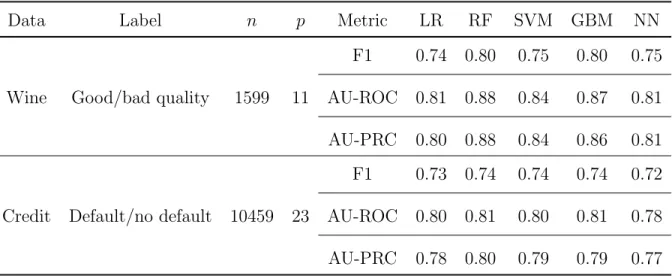
Table 3.1 displays a summary of the datasets and the performance of the trained models. We implement logistic regression with L1 regularization (LR), random forests (RF), support vector machines with RBF kernel (SVM), gradient boosting machines (GBM), and neural networks (NN). High AU-PRC value demonstrates that there is no imbalanced data problem in the two datasets; therefore, we will use AU-ROC value for comparison and refer to it as AUC value in the following text.
Data Label n p Metric LR RF SVM GBM NN
F1 0.74 0.80 0.75 0.80 0.75
Wine Good/bad quality 1599 11 AU-ROC 0.81 0.88 0.84 0.87 0.81
AU-PRC 0.80 0.88 0.84 0.86 0.81
F1 0.73 0.74 0.74 0.74 0.72
Credit Default/no default 10459 23 AU-ROC 0.80 0.81 0.80 0.81 0.78
AU-PRC 0.78 0.80 0.79 0.79 0.77
Table 3.1: Data summary and model performance evaluated by F1 scores, AU-ROC values, and AU-PRC values. Default means failure to repay a loan.
3.1.1 PD Plot and ICE Plot
Partial dependence (PD) plot [Fri01] visualizes the magnitude of feature effects, the shape of the effects, and the complexity of the effects, e.g., linear or nonlinear and monotonic or not.
As defined by Molnar [Mol19], ifX is a row from matrixXn×p withybeing its corresponding label and f represents the function of the original model which predicts E[y|X], partial dependence on feature set S can be denoted as:
fS(XS) = EXC
f(X)=
Z
f(XS, XC)dP(XC), (3.1) where S stands for the feature set on which we would like to see the effects, and C stands for the remaining feature set. It computes the expected value of y at each level of features in set S, when marginalizing over the distribution of other features.
PD plot comes with the constraint of visualizing the effects of a feature set beyond two dimensions. Due to the unseen interaction effects between features, a feature could have bidirectional effects in one dataset, e.g., with half of the data showing positive effects and the other half showing adverse effects [Mol19]. By averaging all positive and negative effects, the PD plot for this feature neutralizes the effects and could become horizontal, concealing its importance. Therefore, we use individual conditional expectation (ICE) plot [GKB15] to detect if interaction effects exist. It complements the PD plot and computes how single predictions, instead of average predictions over all instances in PD plot, change according to feature setS while keeping other features constant. PD plot and ICE plot work together and illustrate the partial dependence on features for both the entire dataset and single instances. To extract the partial dependence values from plots, we use the framework proposed by Britton [Bri19]:
• Given an instance i, one can locate it in a PD plot using its feature value on the x-axis and find the corresponding partial dependence on the y-x-axis. The sum of partial dependence values on all features is the prediction for this instance from the explanation model by PD plots. Suppose Dij is the partial dependence value on feature j for instancei, ˆy∗i can be denoted as:
ˆ yi∗ = p X j=1 Dij. (3.2)
• We make some modifications by dividing continuous feature values into ten discrete bins. We use the median partial dependence value as the dependence value for a bin.
3.1.2 Global Surrogate
Global surrogate method [Mol19] explains the predictions of a black-box model by imitating the black-box model with an interpretable model. It takes the matrix Xn×p as input and the vector of predicted labels of the black-box model ˆyn×1 as the target, and establishes a
surrogate model of E[ˆy|X]. When an interpretable model performs well in predicting the true labelsyn×1, one may prefer to use the model directly with no need to build a surrogate model.
If a black-box model with better performance is needed, a surrogate model could preserve the high accuracy of the black-box model while shedding some light on how it makes the predictions. Many researchers have performed this method using diverse surrogate models [BKB17, TKS16]. In this paper, we implement a decision tree as the global surrogate using
skater1 toolbox based on TREPAN algorithm [Cra96]. Predictions of the surrogate decision tree is ˆyn∗×1.
3.1.3 Global SHAP
Shapley value [Sha53] calculates the contribution of a feature to model predictions while considering all possible subsets of other features. It is the weighted average of differences between predictions with and without this feature [LL17]. As defined by Lundberg and Lee, suppose f is the original model and X is a row from matrix Xn×p, the Shapley value of feature j on observation X can be denoted as:
φj(f, X) = X S⊆{1,···,p}\j |S|!(p− |S| −1)! p! fS∪{j}(XS∪{j})−fS(XS) , (3.3)
where fS(XS) is the model prediction using feature values in set S of observation X while marginalizing over the distribution of other features. Based on Shapley values, SHAP formu-lates an additive explanation model where model predictions are the summation of feature attributions (computed using Shapley values) [LL17]. The explanation model g for
tion X can be denoted as: g(X) =φ0+ p X j=1 φj, (3.4)
whereφ0 is the model prediction with all feature values unknown. It works by adding features
to modelf one at a time and distributing the change in conditional expectationE[f(X)|XS] with and without this newly added feature, instead of fS(XS), to the new feature as its attribution. The feature attributions are SHAP values, and SHAP considers all possible orderings of adding new features [LL17].
For each instance in the dataset, SHAP generates a distinct explanation model g; there-fore, it is a local interpretability method. We implement global SHAP in two ways:
• Visualizing a summary of SHAP values for all instances using shap2 toolbox
• Discretizing the data: Tan et al. [TCH18] computes the global SHAP values by taking the average of all local attributions in g regarding each feature value. To reduce the time and space complexity in computation, we propose grouping each continuous feature into ten discrete bins. We average the local attributions for each bin, instead of each value, and use the discretized global SHAP values to approximate the continuous ones. Suppose ¯φij is the average attribution on featurej for the bin instanceibelonging to, the prediction from the explanation model by global SHAP can be denoted as:
ˆ yi∗ = p X j=1 ¯ φij. (3.5)
Discretization causes information loss to some extent but has two advantages: (1) better in explaining features which are more meaningful after binning, e.g., AverageM-InFile in FICO credit data makes more sense when discretized into ≤ 12 months,
> 12 months and ≤ 24 months, > 24 months than being varying numbers, and (2) scalable when the range of feature values is large.
Another global interpretability method that is model-specific and widely applicable to black-box models is to compute the derivatives of a model function. Many models, e.g., support vector machines with Gaussian kernel and neural networks with sigmoid activation function, have differentiable functions. By computing the first-order partial derivative ∂y∂x and averaging over all instances for each feature value, one can see how a feature affects model predictions. We can also discover the interaction effects between features through calculating the second-order partial derivative ∂∂x2y2. Focusing on model-agnostic interpretablity methods
in this paper, we will not discuss this method in the experiments.
3.2
Analyzing Feature Correlations
Before interpreting the black-box model results, we explore feature correlations, as the in-teraction between features affect how they contribute to the model predictions. In the wine quality data, alcohol (Pearson correlation r= 0.43), sulphates (r= 0.33), and volatile acid-ity (r = −0.32) are most correlated with good-quality red wine. Fixed acidity has high negative correlation with pH (r =−0.71) and positive correlation with density (r = 0.68), which implies that these features affect model predictions through interacting with each other. In the credit data, ExternalRiskEstimate (r = −0.46), NetFractionRevolvingBur-den (r = 0.33), and PercentTradesWBalance (r = 0.26) have the highest correlation with loan default. However, ExternalRiskEstimate and NetFractionRevolvingBurden has negative Pearson correlation of −0.59. Some features also correlate with them, e.g., AverageMInFile with ExternalRiskEstimate (r= 0.34), PercentTradesNeverDelq with ExternalRiskEstimate (r = 0.51), and PercentTradesNeverDelq with NetFractionRevolvingBurden (r = −0.13), which implies that these features may be redundant. PercentTradesWBalance is also corre-lated with ExternalRiskEstimate (r=−0.44) and NetFractionRevolvingBurden (r= 0.55). Considering that there is no perfect multicollinearity and that the features are all meaning-ful, we keep them to preserve as much information as in the datasets. We will compare the correlation results with model explanations. Some of the implemented black-box models, e.g., random forest and XGBoost, can also reduce overfitting through feature selection.
CHAPTER 4
Explaining Wine Quality Predictions
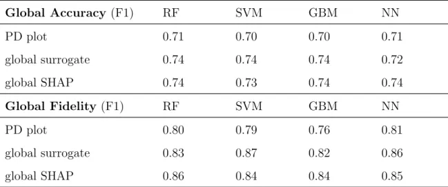
We use the wine quality data to classify if a red wine sample has good quality (quality>5). In Table 3.1, random forest (AUC = 0.88) and gradient boosting machine (AUC = 0.87) achieve the best performance, followed by support vector machine (AUC = 0.84) and neural network with one hidden layer (AUC = 0.81). Table 4.1 presents the global accuracy and fidelity of different explanation models.
Global Accuracy (F1) RF SVM GBM NN PD plot 0.71 0.70 0.70 0.71 global surrogate 0.74 0.74 0.74 0.72 global SHAP 0.74 0.73 0.74 0.74 Global Fidelity (F1) RF SVM GBM NN PD plot 0.80 0.79 0.76 0.81 global surrogate 0.83 0.87 0.82 0.86 global SHAP 0.86 0.84 0.84 0.85
Table 4.1: Global accuracy and fidelity (both measured with F1 score) of the explanation models in predicting good-quality red wine
There are three questions to answer when we compare the results of different global interpretability methods:
1. Which method achieves the best performance in terms of global accuracy and fidelity? 2. Do the methods generate different explanations in terms of feature importance, effect
3. Will the answers for the above two questions change when we switch to a different black-box model?
4.1
PD Plot and ICE Plot Explanations
It has the lowest accuracy and fidelity among the three methods, which is true for all four models. Although RF and GBM perform better than SVM and NN on the data, the accuracy and fidelity of the explanation models are stable across the four models. It also shows a clear drop in predictive power when we use explanation models for prediction, e.g., from RF of F1 = 0.80 to RF explanation model of F1 = 0.71.
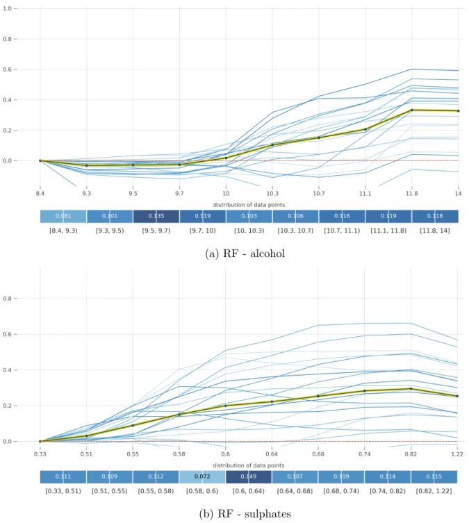
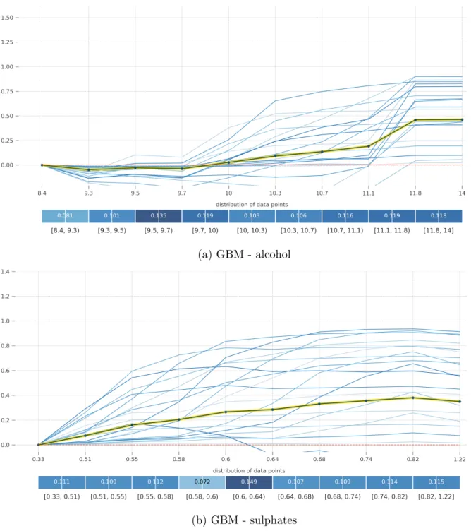
In the PD plots of the four black-box models, alcohol and sulphates are the two most important features for each model. The direction of effects is also consistent, but the magni-tude of effects, computed as partial dependence and visualized by the plot shape, is different for the four models. In Figure 4.1-4.4, the ICE plots reveal the existence of interaction effects between features. For example, in the ICE plot of alcohol by GBM, most clusters of instances experience an increase in probability Pr(quality = good) when alcohol ≈ 11.8, but for instances that already have a high probability when alcohol ≈ 10.3 the increase in probability is negligible when alcohol changes to 11.8.
(a) RF - alcohol
(b) RF - sulphates
Figure 4.1: PD plot and ICE plot for alcohol and sulphates by RF on the wine quality data. The y-axis represents Pr(quality = good). The yellow line is PD plot. Each blue line represents the ICE plot of a cluster of instances, with 20 clusters in total. Each blue bin displays the percentage of instances whose feature value falls into the range.
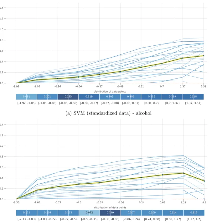
(a) SVM (standardized data) - alcohol
(b) SVM (standardized data) - sulphates
Figure 4.2: PD plot and ICE plot for alcohol and sulphates by SVM on the wine quality data after standardization
(a) GBM - alcohol
(b) GBM - sulphates
Figure 4.3: PD plot and ICE plot for alcohol and sulphates by GBM on the wine quality data
(a) NN (standardized data) - alcohol
(b) NN (standardized data) - sulphates
Figure 4.4: PD plot and ICE plot for alcohol and sulphates by NN on the wine quality data after standardization
4.2
Global Surrogate Explanations
Its accuracy and fidelity are higher than the explanation model by PD plot and ICE plot, which is true for all four models. The accuracy is stable, but a surrogate tree model approx-imates SVM and NN better with higher fidelity than RF and GBM. The predictive power decreases when we use explanation models for prediction by RF and GBM, e.g., from GBM of F1 = 0.80 to GBM explanation model of F1 = 0.74, but does not change much by SVM and NN, e.g., from SVM of F1 = 0.75 to SVM explanation model of F1 = 0.74.
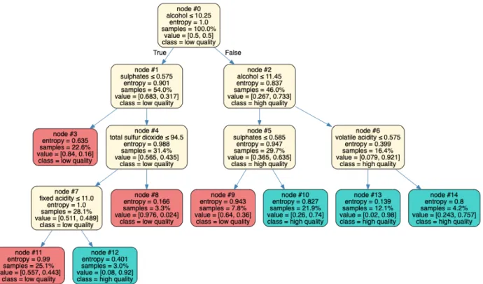
Figure 4.5-4.7 display the structure of the surrogate tree models. Through calculating the reduction in Gini impurity or entropy, we find alcohol, sulphates, and volatile acid-ity are the three most important features for all four models. This matches the result of feature correlation analysis. Surrogate tree models do not show the direction of effects as explicitly as in PD plot, but they uncover interaction effects between features and display a straightforward path towards predictions. For example, in the surrogate tree for RF, when alcohol ≤ 10.25 and sulphates ≤ 0.575, the red wine has 84% chance to have bad quality. When alcohol > 11.45 and volatile acidity ≤ 0.575, the red wine has 98% chance to have good quality.
Figure 4.5: Surrogate tree model for RF on the wine quality data. Surrogate tree model for GBM is the same.
4.3
Global SHAP Explanations
It has the highest accuracy and fidelity overall among the three methods. Similar to the PD plot results, the accuracy and fidelity of the explanation models are stable across the four models. The accuracy of around 0.74 is similar to the accuracy in the global surrogate. The fidelity is 2%−3% higher than or close to the fidelity in the global surrogate, except SVM. In Figure 4.8, alcohol, sulphates, volatile acidity are the three most important features for each model. The direction of effects are: high alcohol, high sulphates, and low volatile acidity increase the probability Pr(quality = good).
Figure 4.9-4.12 present the SHAP dependence plots for the four models. The dependence plots supplement Figure 4.8 by visualizing the complexity of feature effects in terms of linearity and monotonicity. They also reveal interaction effects between features, and the interactions are displayed more clearly on standardized data by SVM and NN. For example, in Figure 4.12, free sulfur dioxide interacts with alcohol most. High alcohol lowers the effect free sulfur dioxide has on Pr(quality = good) when free sulfur dioxide is small but lifts it when free sulfur dioxide is large. The interaction effects shown in the dependence plots are also different across the four models, which means that the four models function differently.
(a) RF (b) SVM
(c) GBM (d) NN
Figure 4.8: SHAP summary plot for RF, SVM, GBM, and NN on the wine quality data. Each point represents an instance. Being red means having a high feature value. Features are ranked by the total magnitude of SHAP values on all instances in descending order. The x-axis states the magnitude of effects and the direction of effects for each instance.
Figure 4.9: SHAP dependence plot for RF on the wine quality data. Each point represents an instance, and each plot is the dependence plot of the feature on the x-axis when using SHAP values. The right y-axis states the feature that correlates with the feature on the x-axis most. Being red means having a high value in the feature on the right y-axis.
CHAPTER 5
Explaining Credit Predictions
We use the credit data to classify whether an applicant will fail to repay the loan (RiskPer-formance = Bad). In Table 3.1, random forest (AUC = 0.81), support vector machine (AUC = 0.80), and XGBoost (AUC = 0.81) achieve the best performance, followed by neu-ral network with two hidden layers (AUC = 0.78). Table 5.1 presents the global accuracy and fidelity of different explanation models. When comparing the results, we answer the same questions proposed when analyzing the wine quality data, in terms of choice of the best interpretability method and the consistency in explanations across different methods and models. Global Accuracy (F1) RF SVM XGB NN PD plot 0.70 0.66 0.72 0.67 global surrogate 0.72 0.72 0.72 0.71 global SHAP 0.73 0.73 0.73 0.72 Global Fidelity (F1) RF SVM GBM NN PD plot 0.84 0.76 0.86 0.74 global surrogate 0.90 0.89 0.91 0.83 global SHAP 0.93 0.91 0.91 0.86
Table 5.1: Global accuracy and fidelity (both measured with F1 score) of the explanation models in predicting loan default
5.1
PD Plot and ICE Plot Explanations
Similar to the results of wine quality data, it has the lowest accuracy and fidelity among the three methods. Although the model performance is close, the accuracy of the explanation models for SVM and NN is lower than that for RF and XGB by 4%. The fidelity is also lower by 8%− 10%. It also shows a drop in predictive power when we use explanation models for prediction, e.g., from SVM of F1 = 0.74 to SVM explanation model of F1 = 0.66. When searching for the most important features by looking at the 23 PD plots, we find that features have various shapes and that it is more difficult than in the wine quality data to identify the top important features through the shapes, since pcredit> pwine.
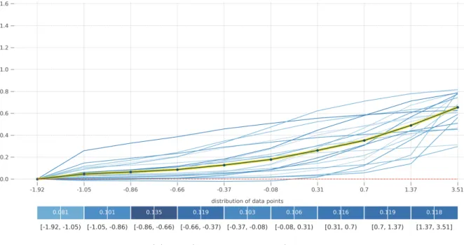
ExternalRiskEstimate and NetFractionRevolvingBurden both show significant effects, and Figure 5.1-5.4 display their PD plots and ICE plots. The direction of effects is approxi-mately consistent, but the magnitude of effects visualized by the plot shape is different across the four models. There also exist interaction effects between features. For example, in the ICE plot of ExternalRiskEstimate by NN, most clusters of instances experience a decrease in probability Pr(RiskPerformance = Bad) when ExternalRiskEstimate ≈ −1.22, but for instances which already have a high probability of default when ExternalRiskEstimate≈ −3 the increase in ExternalRiskEstimate causes a increase in probability instead, not a decrease.
(a) RF - ExternalRiskEstimate
(b) RF - NetFractionRevolvingBurden
Figure 5.1: PD plot and ICE plot for ExternalRiskEstimate and NetFractionRevolvingBur-den by RF on the credit data. The y-axis represents Pr(RiskPerformance = Bad).
(a) SVM (standardized data) - ExternalRiskEstimate
(b) SVM (standardized data) - NetFractionRevolvingBurden
Figure 5.2: PD plot and ICE plot for ExternalRiskEstimate and NetFractionRevolvingBur-den by SVM on the credit data after standardization
(a) XGB - ExternalRiskEstimate
(b) XGB - NetFractionRevolvingBurden
Figure 5.3: PD plot and ICE plot for ExternalRiskEstimate and NetFractionRevolvingBur-den by XGB on the credit data
(a) NN (standardized data) - ExternalRiskEstimate
(b) NN (standardized data) - NetFractionRevolvingBurden
Figure 5.4: PD plot and ICE plot for ExternalRiskEstimate and NetFractionRevolvingBur-den by NN on the credit data after standardization
5.2
Global Surrogate Explanations
Its accuracy and fidelity are higher than the explanation model by PD plot and ICE plot, which is true for all four models. The accuracy is stable, and the predictive power does not decrease much when we use explanation models for prediction, e.g., from SVM of F1 = 0.74 to SVM explanation model of F1 = 0.72. A surrogate tree model approximates NN with lower fidelity than other models.
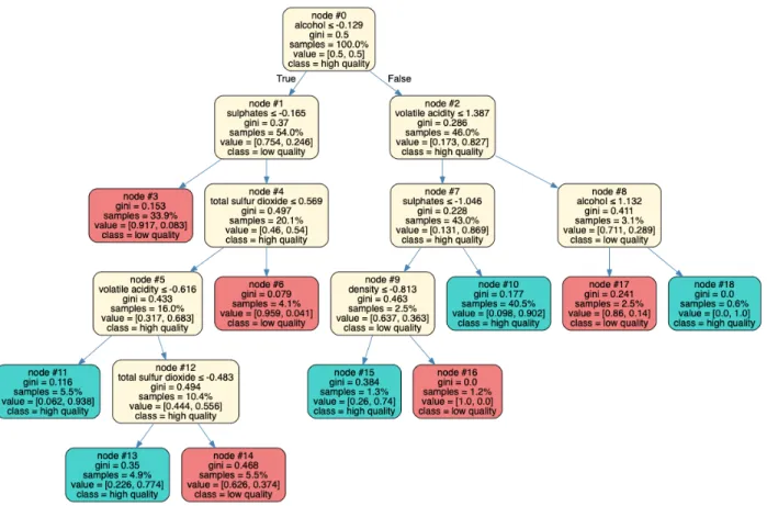
Figure 5.5-5.8 present the structure of the surrogate tree models. After calculating the information gain for each node, we find that ExternalRiskEstimate is the most im-portant feature for all four models, but the models disagree on the rank of other impor-tant features. For RF, AverageMInFile is the second most imporimpor-tant feature, followed by MSinceMostRecentInqexcl7days. For SVM, XGB, and NN, NumSatisfactoryTrades is the second important feature. However, the surrogate tree models share some similar deci-sion paths. For example, in the surrogate tree of RF1, if ExternalRiskEstimate ≤ 76.5 and NumSatisfactoryTrades ≤ 22.5 and AverageMInFile ≤ 65.5, this person has 68.4% probability of not repaying the loan. Similarly, in the surrogate tree of NN (on standard-ized data), if ExternalRiskEstimate ≤ −0.356 and NumSatisfactoryTrades ≤ 0.035 and AverageMInFile≤ −0.064, this person has 83.8% probability of not repaying the loan.
1Note that one split node is MSinceMostRecentInqexcl7days≤ −7.5. Being less than −7.5 means that
this person has not inquired before, therefore the month since the most recent inquiry appears negative. Such a value lowers the probability of loan default, and the surrogate tree reflects the direction of effect correctly. When the split node is true, this person has 63.5% probability of repaying the loan, otherwise 90.4% probability of not repaying the loan.
Figure 5.5: Surrogate tree model for RF on the credit data
Figure 5.7: Surrogate tree model for XGB on the credit data
5.3
Global SHAP Explanations
It has the highest accuracy and fidelity among the three methods, which is true for all four models. The accuracy of 0.73 and fidelity of around 0.92 are also stable, except for NN explanation model (fidelity = 0.86). In Figure 5.9, the rank of the most impor-tant features are slightly different for the four models. NetFractionRevolvingBurden is always one of the three most important features. ExternalRiskEstiamte is the most im-portant feature for RF and XGB, corresponding to PercentTradesNeverDelq for SVM and NetFractionRevolvingBurden for NN. The direction of effects are: high NetFractionRevolv-ingBurden, low ExternalRiskEstiamte, and low PercentTradesNeverDelq increase the prob-ability Pr(RiskPerformance = bad).
Figure 5.10 displays the SHAP dependence plots of the three most important features for each model. It shows that these important features tend to interact with each other, e.g., Av-erageMInFile correlates with ExternalRiskEstimate most in RF and ExternalRiskEstimate correlates with NumSatisfactoryTrades most in NN. It also explains why PercentTradesN-everDelq, instead of ExternalRiskEstimate or NetFractionRevolvingBurden, is the most im-portant feature for SVM: PercentTradesNeverDelq interacts with NetFractionRevolvingBur-den in a way that high NetFractionRevolvingBurNetFractionRevolvingBur-den lowers the effect of PercentTradesN-everDelq when PercentTradesNPercentTradesN-everDelq is small but lifts it when PercentTradesNPercentTradesN-everDelq is large. The feature correlations are also revealed in the correlation analysis.
(a) RF (b) SVM
(c) XGB (d) NN
(a) RF - ExtRskEst, NtFracRevBd, AvgMInF
(b) SVM (standardized data) - PctTrdNevDelq, NtFracRevBd, NInqLst6M
(c) XGB - ExtRskEst, MScMstRctInq, NtFracRevBd
(d) NN (standardized data) - NtFracRevBd, ExtRskEst, NSatTrd
Figure 5.10: SHAP dependence plot of the three most important features for RF, SVM, XGB, and NN on the credit data
CHAPTER 6
Conclusion
In the experiments, we test three global interpretability methods on four nonlinear black-box models using two datasets. We develop a comprehensive understanding of the characteristics of the methods and can develop a strategy to choose from the global interpretability methods using the experiment results.
6.1
Advantages and Disadvantages
We conclude that global interpretability methods have their advantages and disadvantages.
PD plot and ICE plot. PD plot can create unrealistic value combinations when cal-culating the marginal effect of a feature due to the independence assumption. It can also neutralize significant effects when subsets of a dataset show different effect directions [Mol19]. Here we list the strengths and weaknesses revealed in our experiments.
• Strengths: (1) providing a clear visualization of the magnitude, direction, and com-plexity about linearity and monotonicity of feature effects.
• Weaknesses: (1) inefficient in searching for the most important features when the number of features is large, (2) low accuracy of the explanation model due to ignorance of interaction effects, (3) although ICE plot provides insight of underlying interaction effects, it does not identify which two effects interact with each other unless we carry out an exhaustive search of all possible feature combinations.
Global surrogate. There is no guarantee of how close a surrogate tree model can mimic a nonlinear black-box model [HG18]. This method has shown its strengths and weaknesses in our experiments.
• Strengths: (1) identifying interaction effects between features clearly and straightfor-wardly, (2) presenting feature importance in various ways including depth in the tree, frequency of being used for splitting, information gain.
• Weaknesses: (1) implicit in showing the magnitude, direction, and complexity of fea-ture effects, (2) medium accuracy and fidelity of the explanation model.
Global SHAP. SHAP quantifies the contribution of each feature and formulates an addi-tive explanation model that serves as reason codes [HG18]. Generally used in credit scoring and applicable in other fields, reason codes state the reasons why a model generates a spe-cific prediction. However, since SHAP is a local interpretability method, it is not optimized for global explanations after aggregation [TCH18]. In our experiments, it has the following strengths and weaknesses.
• Strengths: (1) high accuracy and fidelity of the explanation model, (2) providing com-prehensive explanations in respect of the magnitude, direction, and complexity of fea-ture effects and the interaction effects between feafea-tures.
• Weaknesses: (1) computationally slow when we use KernelSHAP.
6.2
Towards a Selection Strategy
We conclude that global interpretability methods behave differently on different datasets and black-box models. We answer the questions proposed in Section 4 and develop a strategy that selects the most appropriate method given a new black-box model on a new dataset.
Does the data matter? If we only look at the data, global SHAP achieves the best performance with the highest accuracy and fidelity regardless of what kind of model we use, followed by a global surrogate. This rank is valid for both wine quality data and credit data. However, the methods tend to have higher fidelity for models with more mediocre performance, which is demonstrated by the overall higher fidelity in credit data than the fidelity in wine quality data. Besides, the explanation models may have an upper limit in their accuracy of predicting true labels.
Does the model matter? In most cases, we not only know the data but also are informed of the best model to use. We can pick the most appropriate global interpretability method for the selected model based on fidelity, and fidelity correlates with both model types and model performance.
1. The explanation model of a PD plot and ICE plot generates stable fidelity in most cases, but it is not very faithful when the PD plot is too horizontal. Consider the low accuracy and fidelity for SVM in credit data. Although SVM performs as well as RF, its PD plot is close to horizontal, leading to the summation of dependence values ˆy∗
being similar in two classes.
2. Global surrogate is not suitable for models with too deep or complex structures. Con-sider the high fidelity for SVM and NN in wine quality data and the low fidelity for NN in credit data. They all perform worse than other models. However, due to the small number of features in wine quality data, SVM and NN are relatively simple, but NN in credit data has a more complex layout that cannot be easily imitated by a tree. 3. Global SHAP can achieve high fidelity for different models, no matter how well the models perform. SVM in wine quality data has a lower F1 score and AUC value than RF, but they share close fidelity scores.
Do the explanations differ? The explanations generated by different global interpretabil-ity methods for the same model are consistent. Although the rank of most significant features
is slightly different in credit data, PD plot and global SHAP agree on the direction and shape of feature effects; global surrogate and global SHAP agree on the revealed interaction effects. Second, the explanations can differ in equally good models. In credit data, MSinceMostRe-centTradeOpen and PercentInstallTrades have different magnitudes and shapes of effects for RF and XGB by PD plot; the depth of the surrogate trees are different; the most correlated features by global SHAP are also divergent across the models. When a loss function has multiple optimal solutions, models with different feature weights can achieve equally good performance [Bre01b, HG18]. We can, however, exploit this phenomenon and use the global interpretability methods to choose from all good models for a desirable explanation [HG18] that matches industry expectations best.
What is the selection strategy? When a simple, interpretable model solves a problem appropriately, the direct interpretation of the model is valid and reasonable. In other cases, first, we investigate the data. If features correlate with each other, avoid using PD plot to establish an explanation model; use global surrogate and ICE plot to understand the interaction effects. Second, we identify the interpretation needs. For example, in credit scoring, customers need to know why their loan applications are declined. It could be due to payment delinquencies or other reasons, and the reasons are called reason codes. If the goal is to generate reason codes, go with SHAP. If the goal is to visualize how a prediction is made, a global surrogate tree may be enough. Third, we accordingly mix interpretability methods based on the trained models. Considering the discovered limitations of the three methods, we may also seek local or model-specific interpretability methods for explanations.
6.3
Further Discussions
In this paper, we explain why nonlinear black-box models are hard to interpret, introduce three global interpretability methods, and present a strategy that selects the most appro-priate technique for future tasks. One limitation of the study is that we only test three global interpretability methods, but in practice, a data scientist looks at other
interpretabil-ity methods or combines more than one method for explanations, e.g., permutation feature importance [Bre01a, Mol19] and LIME [RSG16]. Since we have developed a machine learn-ing pipeline for evaluatlearn-ing them, we will continue explorlearn-ing new methods and extendlearn-ing the experiments. A few aspects that deserve further investigation are also listed below.
6.3.1 Faithfulness of Explanations
In the previous study, we use global accuracy and fidelity to measure the performance of explanation models quantitatively, but the faithfulness of explanations lacks examination. In other words, it is unclear to what extent the explanations of a black-box model approximate the ground truth. When there is a benchmark model or a scorecard, which clearly states the most important features and their weights, we can compare our explanations with the truth and decide whether our explanations are trustworthy. However, in most cases, we do not have such preliminary knowledge.
To obtain more understanding about whether the explanations align with the truth, we can set the interaction effects between features manually and simulate a synthetic dataset. The simulation work has two advantages: (1) there are many variations in setting the distri-bution of features, the interaction effects, and the relationship between features and labels. The flexibility in simulation allows many possibilities when we carry out tests of faithfulness since we know how the data is fetched, and (2) it is exciting to see how black-box models gradually outperform white-box models when we loosen the restrictions on the feature as-sumptions during the simulation process. As described by Molnar [Mol19], it is more attrac-tive to interpret “assumption-free black box models” than “assumption-based transparent models,” especially when we have big data from the real world and there is no assumption.
6.3.2 Interpretability on Image Data and Neural Networks
As shown in Table 4.1 and 5.1, neural networks do not perform as well as other algorithms in wine quality data and credit data. Its unsatisfactory performance is reasonable since compared with other algorithms, e.g., random forest, neural networks usually need more data
to achieve the same level of accuracy, but when the data is big enough, it can have outstanding performance. Also, when the features are only meaningful when analyzed together, which is the case in image data, the interpretability methods that calculate independent feature importance or visualize how a prediction is made through a tree are no longer insightful. This brings some other global interpretability methods designed specifically for neural networks which are gradient-based to the stage, e.g., model distillation [TCH18, Mol19], saliency maps [SVZ13, AJ18, MJ18], integrated gradients [STY17, AJ18, MJ18], and occlusion sensitivity [ZF14, AJ18, MJ18].
REFERENCES
[AB18] Amina Adadi and Mohammed Berrada. “Peeking inside the black-box: A survey on Explainable Artificial Intelligence (XAI).” IEEE Access,6:52138–52160, 2018. [AJ18] David Alvarez-Melis and Tommi S Jaakkola. “On the robustness of interpretability
methods.” arXiv preprint arXiv:1806.08049, 2018.
[BKB17] Osbert Bastani, Carolyn Kim, and Hamsa Bastani. “Interpretability via model extraction.” arXiv preprint arXiv:1706.09773, 2017.
[Bre01a] Leo Breiman. “Random forests.” Machine learning,45(1):5–32, 2001.
[Bre01b] Leo Breiman et al. “Statistical modeling: The two cultures (with comments and a rejoinder by the author).” Statistical science,16(3):199–231, 2001.
[Bri19] Matthew Britton. “VINE: Visualizing Statistical Interactions in Black Box Mod-els.” arXiv preprint arXiv:1904.00561, 2019.
[CCA09] Paulo Cortez, Ant´onio Cerdeira, Fernando Almeida, Telmo Matos, and Jos´e Reis. “Modeling wine preferences by data mining from physicochemical properties.”
Decision Support Systems, 47(4):547–553, 2009.
[Cra96] Mark W Craven. “Extracting comprehensible models from trained neural net-works.” Technical report, University of Wisconsin-Madison Department of Com-puter Sciences, 1996.
[DG17] Dheeru Dua and Casey Graff. “UCI Machine Learning Repository.”, 2017. http: //archive.ics.uci.edu/ml.
[DK17] Finale Doshi-Velez and Been Kim. “Towards a rigorous science of interpretable machine learning.” arXiv preprint arXiv:1702.08608, 2017.
[FIC18] FICO. Explainable machine learning challenge, 2018. https://community.fico. com/s/explainable-machine-learning-challenge.
[Fre14] Alex A Freitas. “Comprehensible classification models: a position paper.” ACM SIGKDD explorations newsletter, 15(1):1–10, 2014.
[Fri01] Jerome H Friedman. “Greedy function approximation: a gradient boosting ma-chine.” Annals of statistics, pp. 1189–1232, 2001.
[GKB15] Alex Goldstein, Adam Kapelner, Justin Bleich, and Emil Pitkin. “Peeking inside the black box: Visualizing statistical learning with plots of individual conditional expectation.” Journal of Computational and Graphical Statistics, 24(1):44–65, 2015.
[GMR18] Riccardo Guidotti, Anna Monreale, Salvatore Ruggieri, Franco Turini, Fosca Gi-annotti, and Dino Pedreschi. “A survey of methods for explaining black box models.” ACM computing surveys (CSUR),51(5):1–42, 2018.
[HG18] Patrick Hall and Navdeep Gill. Introduction to Machine Learning Interpretability. O’Reilly Media, Incorporated, 2018.
[LL17] Scott M Lundberg and Su-In Lee. “A unified approach to interpreting model predictions.” In Advances in neural information processing systems, pp. 4765– 4774, 2017.
[MJ18] David Alvarez Melis and Tommi Jaakkola. “Towards robust interpretability with self-explaining neural networks.” In Advances in Neural Information Processing Systems, pp. 7775–7784, 2018.
[Mol19] Christoph Molnar. Interpretable Machine Learning. 2019. https://christophm. github.io/interpretable-ml-book/.
[NJK19] Harsha Nori, Samuel Jenkins, Paul Koch, and Rich Caruana. “InterpretML: A Unified Framework for Machine Learning Interpretability.” arXiv preprint arXiv:1909.09223, 2019.
[RSG16] Marco Tulio Ribeiro, Sameer Singh, and Carlos Guestrin. ““ Why should i trust you?” Explaining the predictions of any classifier.” In Proceedings of the 22nd ACM SIGKDD international conference on knowledge discovery and data mining, pp. 1135–1144, 2016.
[Sha53] Lloyd S Shapley. “A value for n-person games.” Contributions to the Theory of Games, 2(28):307–317, 1953.
[STY17] Mukund Sundararajan, Ankur Taly, and Qiqi Yan. “Axiomatic attribution for deep networks.” In Proceedings of the 34th International Conference on Machine Learning-Volume 70, pp. 3319–3328. JMLR. org, 2017.
[SVZ13] Karen Simonyan, Andrea Vedaldi, and Andrew Zisserman. “Deep inside convo-lutional networks: Visualising image classification models and saliency maps.”
arXiv preprint arXiv:1312.6034, 2013.
[TCH18] Sarah Tan, Rich Caruana, Giles Hooker, Paul Koch, and Albert Gordo. “Learn-ing global additive explanations for neural nets us“Learn-ing model distillation.” arXiv preprint arXiv:1801.08640, 2018.
[TKS16] Jayaraman J Thiagarajan, Bhavya Kailkhura, Prasanna Sattigeri, and Karthikeyan Natesan Ramamurthy. “TreeView: Peeking into deep neural net-works via feature-space partitioning.” arXiv preprint arXiv:1611.07429, 2016. [ZF14] Matthew D Zeiler and Rob Fergus. “Visualizing and understanding convolutional
networks.” In European conference on computer vision, pp. 818–833. Springer, 2014.