Parameter identification in Choquet Integral by the
Kullback-Leibler diversgence on continuous densities
with application to classification fusion.
Emmanuel Ramasso, Sylvie Jullien
To cite this version:
Emmanuel Ramasso, Sylvie Jullien.
Parameter identification in Choquet Integral by the
Kullback-Leibler diversgence on continuous densities with application to classification fusion..
European Society for Fuzzy Logic and Technology, EUSFLAT - LFA’11., Jul 2011,
Aix-Les-Bains, France. sur cl´
e USB, pp.1-8, 2011.
<
hal-00603967
>
HAL Id: hal-00603967
https://hal.archives-ouvertes.fr/hal-00603967
Submitted on 27 Jun 2011
HAL
is a multi-disciplinary open access
archive for the deposit and dissemination of
sci-entific research documents, whether they are
pub-lished or not.
The documents may come from
teaching and research institutions in France or
abroad, or from public or private research centers.
L’archive ouverte pluridisciplinaire
HAL
, est
destin´
ee au d´
epˆ
ot et `
a la diffusion de documents
scientifiques de niveau recherche, publi´
es ou non,
´
emanant des ´
etablissements d’enseignement et de
recherche fran¸
cais ou ´
etrangers, des laboratoires
publics ou priv´
es.
Parameter identification in Choquet Integral by
the Kullback-Leibler divergence on continuous
densities with application to classification fusion
Emmanuel Ramasso
1Sylvie Jullien
21FEMTO-ST Institute, UMR CNRS 6174 - UFC / ENSMM / UTBM, AS2M Dep., 25000 Besançon, France 2Dynamic3D, Route de Demigny, 71102 Chalon-Sur-Saône, France
Abstract
Classifier fusion is a means to increase accuracy and decision-making of classification systems by design-ing a set of basis classifiers and then combindesign-ing their outputs. The combination is made up by non lin-ear functional dependent on fuzzy measures called Choquet integral. It constitues a vast family of ag-gregation operators including minimum, maximum or weighted sum. The main issue before applying the Choquet integral is to identify the 2M −2 pa-rameters for M classifiers. We follow a previous work by Kojadinovic and one of the authors where the identification is performed using an information-theoritic approach. The underlying probability den-sities are made smooth by fitting continuous para-metric and then the Kullback-Leibler divergence is used to identify fuzzy measures. The proposed framework is applied on widely used datasets.
Keywords: Information fusion, Fuzzy measures, Relative Entropy, Health assessment, Classification
1. Introduction
In most of pattern recognition tasks, a first step consists in extracting relevant features bringing in-formation on classes of interest. Features are then transformed into membership degrees according to the different classes by entities called classifiers.
A classifier is a system that takes as inputs aQ -dimensional vectorXt= [x
1. . . xQ] (also called
fea-tures or attributes) and generates a degree of confi-dence in the statement "X belongs to class ωj" for
all classes in Ω ={ω1. . . ωK}.
Multiple Classifier Systems (MCS) [1] are de-signed when complementary (and sometimes re-dundant) information sources (here classifiers) are used in order to improve classification accuracy and decision-making. MCS can be also viewed as in-formation fusion systems where inputs are classi-fiers. MCS can take several forms and among them the parallel one which takes as inputM ×K par-tial degrees of confidence and generates an output, called global confidence degree, made up of K de-grees of confidence (one for each class). We denote byφm,j(X) the degree of confidence delivered by a
classifier m∈ {1. . . M} for classωj ∈ Ω given the
observationX.
Usual combinations of classifier outputs include product, naive Bayes and decision templates among others [1] but most of them can be used provided each output represents an independent source of in-formation. However, the independance assumption is not always satisfied. To face this problem, an approach that considers interactions among classi-fier outputs such as fuzzy integrals and in particular the Choquet Integral [2, 3] can be used. The explicit interaction coefficients (in the 2-additive form) pro-vide very interesting information on complementar-ity and redundancy of the fused data which can also be used for subset selection [4].
A fuzzy integral is a type of non-linear func-tional dependent on fuzzy measures which consti-tutes a vast family of aggregation operators includ-ing many widely used operators (minimum, maxi-mum, weighted sum, ordered weighted sum and so on) [5]. In order to be combined by the Choquet Integral, the commensurability [6] of classifier out-puts must be satisfied. That means the classifier outputs must be defined on the same measurement scale.
The combination of all partial confidence degrees provided by classifiers is thus made up by a Choquet Integral which is described in the next section.
2. Choquet capacities and Choquet Integral
Let the M classifiers (sources) be denoted by Θ =
{θ1, θ2. . . θM}. A fuzzy measureµkfor a given class
ωkweighs the importance of a subset of sourcesS⊆
Θ and is defined by [2, 3]:
µk : 2Θ → [0,1]
S 7→ µk(S)
(1) satisfying the following constraints:
• µk(∅) = 0 and µk(Θ) = 1
• S⊆T ⇒µk(S)≤µk(T) (monotonicity)
The fuzzy measure is said:
• additive when µk(S ∪ T) = µk(S) +µk(T),
∀S, T ⊆Θ/S∩T =∅ (probability measure),
• super-additivewhenµk(S∪T)≥µk(S)+µk(T),
• sub-additivewhenµk(S∪T)≤µk(S) +µk(T),
∀S, T ⊆Θ/S∩T =∅.
In classification problems, the fuzzy measure is used in order to take into account interactions between sources. One fuzzy measure is tuned for each class and each discrete Choquet Integral aggregates the information provided by the sources as follows [2, 3]:
C(φ1, . . . , φM) = M
X
i=1
(φ(i)−φ(i−1))·µk(S(i)) (2)
whereµk(S(i)) is the importance of subset of sources
S(i)={θ(i), ..., θ(M)} and the valueφ(i) is provided
by sourceθ(i). The notation (.) indicates a
permu-tation of indices according to the values provided by the sources such asφ(1)≤φ(2)≤... ≤φ(M)≤1 (and by convention φ(0) = 0). The Choquet
inte-gral thus coincides to the weighted arithmetic mean when the fuzzy measure is additive.
One approximation of Eq. 2 called 2-additive Choquet Integral is often used and consists in con-sidering a 2-order additive capacity which takes into account both the weights of each source and the in-teraction between pairs. The weightνi of a source
θi(for the detection of classωk) and the coefficient
Iijof interaction between both sourcesθiandθjcan
be obtained from the fuzzy measureµk by [2, 3]:
νi= X T⊆Θ\i (M − |T| −1)!|T|! M! × µk(T∪ {i})−µk(T) (3a) Iij = X T⊆Θ\{i,j} (M− |T| −2)!|T|! (M−1)! × µk(T∪ {i, j})− µk(T∪ {i})−µk(T∪ {j}) +µk(T) (3b) These parameters are interesting for interpreting the fuzzy measure and also to highlight which sources are important and how they interact. When interactions between two sources are positive, the sources are said complementary while they are said redundant when interactions are negative.
The problem of Choquet Integral parameters identification was treated by several authors [4, 7]. In the context of classification as considered here (where the classes are known), the method pro-posed by Grabisch [3] and called Heuristic Least Mean Square (HLMS) is often used. However it re-quires the global scores (the real output of the Cho-quet Integral) to perform the optimization of the fuzzy measure. Recently, two information theoritic methods based on entropy [8, 6] and on relative en-tropy [9] were proposed. The former is purely unsu-pervised and requires only degrees of confidence of classifiers while the latter requires the ground truth, i.e. the real class of each pattern. The relative
entropy-based approach is supervised but requires less prior information than HLMS.
3. Identification of Choquet Integral parameters based on discrete relative entropy
3.1. A probabilistic view
Each fuzzy valueµk(S) expresses the relative
impor-tance of a subsetS for distinguishing classωk from
the others [8, 6]. In order to identify them, the au-thors in [9] proposed to use the relative entropy, also called Kullback-Leibler divergence (KL) [10], which is a measure of divergence between two densities. It could be interpreted as the expected discrimina-tion informadiscrimina-tion between two hypotheses and thus appears very natural for the identification of fuzzy measures.
To compute KL, one needs first to compute:
• the distribution (sayPkS) of confidence degrees in classωk conditional to classωk,
• and the distribution (sayPS
k) of confidence
de-grees in classωkconditional to the other classes
(ωk= Ω\ωk),
both given a subset of sources S. These distribu-tions characterize the input data (confidence de-grees) and the greater is the difference (calculated by KL) between them, the higher is the discrimina-tion power.
Identifying fuzzy measure using a probabilistic approach was introduced in [8, 6] where the author proposed an unsupervised entropy-based method. When the class is known for each input pattern, the KL-based approach proposed in [9] should be used. It fully exploits the available information provided by the training dataset and, as expected, increases the discrimination power.
3.2. Relative entropy
We assume all confidence degrees to be com-mensurable values in [0,1] which is generally true in classification. Let PΘ
k (Y) with Y =
(φ1,k(X), φ2,k(X). . . φM,k(X)) ∈ [0,1]|Θ| (resp.
PΘ
k (Y)) be the probability that classifiers 1,2. . . M
jointly provide the values φ1,k(X),φ2,k(X),. . . and
φM,k(X) given the ground truth is class ωk (resp.
given ωk) and observation X. In [9], the
distribu-tions were assumeddiscreteand the relative entropy (KL) of both distributions was thus given by:
D(PkΘ||PkΘ) =X Y PkΘ(Y) logP Θ k (Y) PΘ k (Y) (4)
For the sake of simplicity, we will denote byRk(S)
the KL value given byD(PS
k||PkS) for a given subset
of sourcesS⊆Θ:
Rk(S)≡ D(PkS||P S
Note that when the distributions PΘ
k and PkΘ are
computed, the distributionsPS
k and PkS for S⊂Θ
are obtained by marginalizing out the components
θ∈Θ, θ /∈S.
To compute Eq. 4, the support of the distribution
PS
k must be included in the support of the
distri-bution PS
k otherwise the relative entropy diverges
towards infinity. In order to respect this constraint, the skew divergence was used in [9].
3.3. From relative entropy to Choquet capacities
The relative entropy has to satisfy the conditions presented Section 2 in order to be interpreted as a Choquet capacity. For that, the relative entropy
Rk(S) for a subset S is normalized as in
Kojadi-novic’s method [8, 6] by the entropy of the whole set of sourcesRk(Θ):
µk(S) =
Rk(S)
Rk(Θ)
(6) Moreover, the relative entropy is zero when the setS
is empty but also when both distributions are iden-tical. Therefore, a source that provides the same degrees of support for a sought-after classωk and
for the other classesωkis assigned a low importance
value since it can not distinguish classωk from the
others. This is exactly the mean of discrimination power.
The relative entropy has also to satisfy the mono-tonicity constraint (Section 2), i.e. given two sourcesθiandθj, the relative entropy has to satisfy
the following equations:
µ({θi, θj})≥µ({θi}) (7a)
µ({θi, θj})≥µ({θj}) (7b)
In order to check these constraints, one can rewrite the relative entropy as [11, 8, 6]:
Rk({θi, θj}) =Rk({θi}) +Rk({θj|θi}) (8)
that is always positive and therefore has a mono-tonic behavior [11, 8, 6, 9]:
Rk({θi, θj})≥Rk({θi}) (9a)
Rk({θi, θj})≥Rk({θj}) (9b)
This reasoning can be extended easily to larger sub-sets of sources. Therefore, the normalized relative entropy satisfies all the constraints in order to be interpreted as a Choquet capacity.
3.4. Modeling positive and negative interactions
When sourcesθi andθj, that provide distributions
PS
k and PkS, are independent, the relative entropy
has an additive behavior [11, 8, 6]:
Rk({θi, θj}) =Rk({θi}) +Rk({θj}) (10)
When sources θi and θj are interacting one each
other, the relative entropy can be expressed by:
Rk({θi, θj}) =Rk({θi}) +Rk({θj})
+Rk({θj|θi})−Rk({θj})
(11)
where the last term can be negative or positive ac-cording to sourcesθiandθjimplying that the
iden-tified Choquet capacities can be super-additive or sub-additive. Therefore the proposed method is able to model and identify both positive and neg-ative interactions whereas Kojadinovic’s approach can only identify negative ones.
4. Identification of Choquet Integral parameters based on continuous relative entropy
4.1. On using a continuous approach
The core of the KL-based method is the evalua-tion of the multidimensional probability distribu-tions (PS
k and P S
k). In [8, 6, 9], the distributions
were computed using discretization of confidence degrees (and histograms). We rather propose to remain in the continuous space (the space of the degrees of confidence) and to use parametric con-tinuous densities for confidence degrees modelling. These densities allow to:
• Ensuring an infinite support for the distri-butions and therefore avoiding using artificial methods to solve the problem of minimum sup-port.
• Avoiding the necessity of finding the optimal number of bins for the histograms. This could be a serious problem for high dimensional data such as in image processing or in complex sys-tems diagnosis.
• Obtaining a more precise paving of the input space and therefore generating smooth distri-butions and improving the computation of the relative entropy by summing over more data points sampled from the continuous densities.
• Simplifying the computation of marginaliza-tions (according to the family of densities).
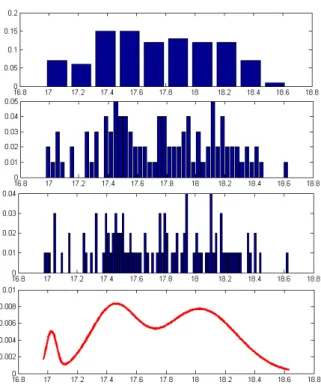
Fig. 1 depicts the problem of finding the num-ber of bins for discrete histograms. We drew 100 points from a mixture of five Gaussians with equal probability and with means 0, 10, 25, 35, 50 and unit variance. We then computed histograms (de-picted in the first three figures) with 10, 50 and 100 bins and we also run an EM in order to identify au-tomatically the parameters of a continuous density made up of five components. The results are very different with a preference given to the last figure.
Figure 1: Role of the number of bins (see comments in the text).
4.2. Modelling inputs by continuous densities
4.2.1. Modelling
We assume that the joint probability density func-tion related toPΘ
k (and similarly forP
Θ
k ) has a
tinuous and parametric form. For example, we con-sider mixtures of Gaussians which are very general and have interesting properties:
PkΘ(Y) = Lk X a=1 ck,a·fk,a(Y) (12) where
fk,a(Y) =N(Y|αk,a,Σk,a) (13)
withY = (φ1,k(X), φ2,k(X). . . φM,k(X))∈[0,1]|Θ|
the joint observation of degrees of confidence,ck,a
the mixing coefficient of component a (among Lk,
with P
ack,a = 1) and N(Y|αk,a,Σk,a) a
multidi-mensional normal density with mean αk,a and
co-variance Σk,a(positive definite):
N(Y|αk,a,Σk,a) = exp−1 2(Y −αk,a) TΣ−1 k,a(Y −αk,a) (2π)M/2|Σ k,a|1/2 (14)
The dimension of the parameters is the same as Θ which isM. The same expression holds forPΘ
k : PkΘ(Y) = Lb X b=1 ck,b·gk,b(Y) (15) with different parameters indexed by subscripts (k, b).
4.2.2. Learning parameters of densities
The parameters of the densities can be esti-mated automatically by standard methods such as the Expectation-Maximization algorithm (EM [12]) where L, the number of components, can also be estimated.
When the parameters of the distributionsPΘ
k and
PΘ
k have been specified, it is easy to computeP S k
and PS
k for subsets S ⊂ Θ by marginalization.
In case the joint density related to PΘ
k is
repre-sented by a mixture of multivariate Gaussians, the marginal is also a mixture of multivariate Gaus-sians where some components (marginalized out) have been eliminated. In particular, the |S| com-ponents of the mean vector of the marginal are the means of the variables inS and its covariance ma-trix is composed of the pairwise covariances of the same variables.
4.3. Continuous relative entropy
For two unimodal multivariate normal densitiesfk
and gk (withLa =Lb = 1), the KL has an exact
closed form [13]: Rexk (S;fk;gk) = 1 2 log |Σ k| |Σk| +. . . TrΣ−1 k Σk −M +. . . µk−µktΣk−1 µk−µk (16)
When densities are multimodal, the continuous rel-ative entropy is obtained by integrating on the sup-port ofPS k, Supp(PkS) ={Y :PkS(Y)>0}: Rk(S) = Z Y∈Supp(PS k) PkS(Y) logP S k(Y) PS k(Y) dY (17) To evaluate this expression, several methods can be used [13]. In this paper, we have used Monte Carlo sampling (MC) and variational approxima-tion (VA).
The MC method consists in drawing samples from the mixture associated toPS
k. For that, a
compo-nent is chosen randomly using the distributionck,..
A continuous sample is then drawn from the asso-ciated Gaussian component and the density is eval-uated. Given{Yi, i= 1. . . N}the set of i.i.d.
sam-pled points, we can approximate the integral (17) by its MC estimate: RMCk (S) = 1 N X i logP S k(Yi) PS k(Yi) → D(PkS||PkS) (18) The precision of the evaluation of KL depends ob-viously on the number of simulations.
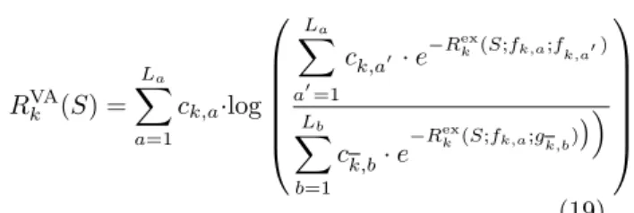
by the following expression [13]: RVAk (S) = La X a=1 ck,a·log La X a0=1 ck,a0 ·e−R ex k(S;fk,a;fk,a0) Lb X b=1 ck,b·e−R ex k(S;fk,a;gk,b) (19) whereRex
k (S;fk,a;gk,b) is the exact value of KL
be-tween component a of fk and component b of gk
given by Eq. 16.
4.4. Final algorithm
The overall algorithm for computing the fuzzy mea-sure is as follows:
Require: Lk the set of confidence degrees in class
ωkof M classifiers given the ground truth is class
ωk
Require: Lk the set of confidence degrees in class
ωk of M classifiers given the ground truth are
classes different fromωk
Ensure: the fuzzy measureµk for classωk
1: PkΘ←Estimate the parameters of the densities onLk
2: PΘ
k ←Estimate the parameters of the densities
onLk
3: µk(Θ)←1,µk(∅)←0
4: Rk(Θ)←Apply Eq. 17 withPkΘ andPkΘ
5: for allS⊂Θdo 6: PS k ←marginalizePkΘ onS 7: PS k ←marginalizeP Θ k onS
8: Rk(S)←Apply Eq. 17 withPkS andPkS
9: µk(S)←
Rk(S)
Rk(Θ)
(Eq. 6) 10: end for
From µk, one can compute the weight of each
source (i.e. classifier) and their interactions using Eq. 3b. These values can help an end-user or any people interested in knowing which classifiers con-tribute to the final results as well as how they in-teract.
5. Experiments
A toy example is first presented. Then, the pro-posed method is evaluated on two datasets from UCI [14]: vehicle and image segmentation. Classi-fiers used were the following: Evidential Neural Net-work (EvNN) [15] (with 4 prototypes for each class), Evidential Nearest Neighborhood (EvKNN) [16] (with K = 5) and Support Vector Machines (SVM) [12] (with a Gaussian Kernel of size 2.2). Classifiers were learnt using 1-vs-1 strategy for each class, and the final scores were obtained by using a weighted vote. SVM scores were transformed into probabilities using a sigmoid transfer function. Note that classifier parameters were not “optimized" for each dataset, since the goal is here to assess the
fusion process. The KL was assessed using the MC method using 1e6 samples.
5.1. A toy example
Figure 2: A densityPkΘ.
Figure 3: A densityPΘ
k.
As an example, let consider two classifiersθ1 and
θ2 with confidence degrees inωk, given the ground
truth is ωk, being distributed according to Fig. 2,
and according to Fig. 3 for confidence degrees inωk
given the ground truth is another class ωk. From
these densities, we are looking for characterizing the importance of the coalition {θ1, θ2} in
distinguish-ingωk from ωk.
In Fig. 2, the confidence degrees of classifier 1 are globally close to unity given classωk. That means
classifier 1 often provides high scores for ωk given
the ground truth isωk. Classifier 2 however seems
to provide some results close to 0.5 meaning classi-fier 2 is frequently not certain about the predicted class. Given the ground truth isωk (Fig. 3),
clas-sifier outputs are globally close to 0 for ωk. That
means classifiers generally provide low values forωk
when the ground truth isωk as expected.
In order to quantify the importance µk({θ1, θ2})
divergence between both distributions. The higher is the divergence, the higher is the importance of
{θ1, θ2}for distinguishingωk from the other classes.
In this example, densities were obtained using two mixtures with the following parameters:
• given ωk, αk,1 = [0.1, 0.1], Σk,1 =
[.01, 8; 8, .01], αk,2 = [0.2, 0.4] and Σk,2 =
[.02, .01; .01, .02] (with equal mixing coeffi-cientsck,a).
• given ωk, αk,1 = [0.8, 0.8], Σk,1= [8, 1; 1, 8],
αk,2 = [0.55, 0.9], Σk,2 = [.02, 8; 8, .02],
αk,3 = [0.95, 0.97], Σk,3 = [4, 1; 1, 4] (with equal mixing coefficients ck,a).
With these parameters, Eq. 17 leads to
Rk({θ1, θ2})≈9.44 (withN = 1.106).
5.2. Vehicle dataset
The UCI’s vehicle dataset is a four-classes problem composed of 946 examples almost uniformly dis-tributed between classes. The goal is to classify data into one of the following types of vehicle: OPEL (ω1), SAAB (ω2), BUS (ω3) and VAN (ω4). The
half of the dataset was used for classifier training, and the other half for testing.
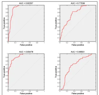
Figure 4: EvNN classification results. Top: classes 1 and 2, bottom: classes 3 and 4.
Figures 4-6 pictorially described ROC curves computed for each class given results of classifiers. Also are displayed the Area Under the Curve (AUC) which reflects the efficiency in detecting the class. These curves can be compared with ROC curves of Figure 7 computed from the results of the fusion process proposed in this paper. Table 1 also gives the obtained fuzzy measures, while interaction and classifier weights computed from them (as detailed previously) are provided in Tables 2 and 3.
ROC curves clearly show the complementarity of individual classifiers. For example, classω1is better
recognized using EvKNN (Fig. 5) with almost 98%
Figure 5: EvKNN classification results. Top: classes 1 and 2, bottom: classes 3 and 4.
Figure 6: SVM classification results. Top: classes 1 and 2, bottom: classes 3 and 4.
Figure 7: Fusion by Choquet Integral. Top: classes 1 and 2, bottom: classes 3 and 4.
of good classification. Classω2 is better recognized
using SVM (Fig. 6) with an accuracy close to 83%. Class ω3 is well recognized (about 93%) by EvNN
(Fig. 4) and EvKNN (Fig. 5). Lastly, class ω4 is
better detected by SVM (Fig. 6).
set ω1 ω2 ω3 ω4 1 0.22 0.39 0.23 0.24 2 0.66 0.57 0.34 0.37 12 0.75 0.70 0.44 0.65 3 0.36 0.29 0.20 0.44 13 0.50 0.60 0.43 0.62 23 0.89 0.84 0.83 0.65
Table 1: The fuzzy measure for each class learnt by the proposed algorithm for the “vehicle" dataset.
set ω1 ω2 ω3 ω4
I12 −0.08 −0.20 −0.10 +0.10
I13 −0.03 −0.02 +0.03 +0.01
I23 −0.08 +0.03 +0.33 −0.10
Table 2: Interaction values associated to the fuzzy measures of Table 1.
set ω1 ω2 ω3 ω4
ν1 0.15 0.26 0.19 0.28
ν2 0.56 0.47 0.45 0.35
ν3 0.29 0.28 0.37 0.37
Table 3: Weight values associated to the fuzzy mea-sure of Table 1.
As shown in Figure 7, the proposed fusion pro-cess draw benefits of all these classifiers, providing AUCs close to 99%, 84%, 97% and 88% for class
ω1,ω2, ω3 and ω4 respectively (improvement close
to 10%). Interaction indexes can explain this re-sult. Indeed, class ω1, that is well detected by all
classifiers, is represented by a fuzzy measure with negative interactions because of redundancy. The highest redundancy is detected for classω2between
EvNN and EvKNN (I12=−0.20) while the highest
complementarity is detected for class ω3 between
EvNN and SVM classifiers (I23= +0.33). Weights
are also the highest for classifiers with the best ac-curacies, except for classω2.
5.3. Image segmentation dataset
The UCI’s image segmentation dataset is a seven-classes problem composed of 210 training exam-ples and 2100 for testing. Initially, features are 19-dimensional but we reduced them to 6 dimensions and we kept features [1 3 4 8 9 17]. The goal is thus to classify data into one of the following types of vehicle: Brickface (ω1), Sky (ω2), Foliage (ω3),
Cement (ω4), Window (ω5), Path (ω6) and Grass
(ω7).
For this dataset, we present the results in the form of confusion matrices (Table 4-7) where the ground truth is on columns while results of classifiers are
class ω1 ω2 ω3 ω4 ω5 ω6 ω7 ω1 0 0 0 6 18 0 0 ω2 67 264 0 67 15 0 0 ω3 0 0 41 8 7 0 0 ω4 233 36 259 219 256 0 0 ω5 0 0 0 0 3 0 0 ω6 0 0 0 0 1 300 1 ω7 0 0 0 0 0 0 299
Table 4: Confusion matrix of EvNN classifier (global acc.: 53.6%, degraded on purpose).
class ω1 ω2 ω3 ω4 ω5 ω6 ω7 ω1 152 9 26 69 61 0 0 ω2 38 223 0 55 17 0 0 ω3 22 1 176 12 45 0 0 ω4 45 55 13 140 6 30 0 ω5 43 12 85 24 171 0 14 ω6 0 0 0 0 0 270 0 ω7 0 0 0 0 0 0 286
Table 5: Confusion matrix of EvKNN classifier (global acc.: 67.5%) class ω1 ω2 ω3 ω4 ω5 ω6 ω7 ω1 98 0 1 3 4 0 0 ω2 4 78 0 3 0 0 0 ω3 5 0 59 0 0 0 0 ω4 18 6 3 49 1 0 0 ω5 0 0 14 0 94 0 0 ω6 0 0 0 0 0 111 0 ω7 175 216 223 245 201 189 300
Table 6: Confusion matrix of SVM classifier (global acc.: 37.6%)
on lines. Tables 4- 6 are confusion matrices of indi-vidual classifiers. We here degraded on purpose the results of the first classifier (EvNN) on classesω1,
ω3, ω5 and ω7 (by adding noise on the parameters
trained by the algorithm). As a result, the confusion matrix presents low detection rate for these classes (close to 0 for some of them). We then applied the fusion process. class ω1 ω2 ω3 ω4 ω5 ω6 ω7 ω1 97 3 3 1 11 0 0 ω2 55 234 0 58 15 0 0 ω3 0 0 156 6 20 0 0 ω4 148 63 62 231 113 3 0 ω5 0 0 79 4 141 0 7 ω6 0 0 0 0 0 297 0 ω7 0 0 0 0 0 0 293
Table 7: Confusion matrix after fusion using MC sampling (global acc.: 69%)
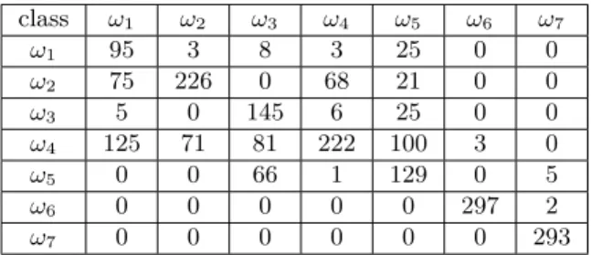
Table 7 shows the confusion matrix of the fusion process result. This matrix clearly shows that the proposed method is able to draw benefits from in-dividual classifiers. Table 8 is the confusion matrix obtained by the fusion process based on the vari-ational approximation of the KL divergence which shows that, for this application, the approximation
class ω1 ω2 ω3 ω4 ω5 ω6 ω7 ω1 95 3 8 3 25 0 0 ω2 75 226 0 68 21 0 0 ω3 5 0 145 6 25 0 0 ω4 125 71 81 222 100 3 0 ω5 0 0 66 1 129 0 5 ω6 0 0 0 0 0 297 2 ω7 0 0 0 0 0 0 293
Table 8: Confusion matrix after fusion using varia-tional approximation (global acc.: 66%)
is satisfying.
Interaction values obtained in this application are shown in Table 9. For classesω1, ω3 and ω5
inter-actions between classifiers emphasize complemen-tarity. In particular, classifiers EvNN and EvKNN present the strongest complementarities. This is represented in confusion matrix where these clas-sifiers mix sometimes several classes while classifier 3 confuses between classω7and the others.
In general, an efficient classifier has also a rela-tively high weight (Tab. 10), and if it is not the case, interaction values provide compensation.
class ω1 ω2 ω3 ω4 ω5 ω6 ω7
I12 0.32 −0.29 0.15 −0.22 0.03 −0.17 −0.28
I13 0.06 0.00 0.06 −0.04 0.03 −0.02 −0.03
I23 −0.09 0.07 0.02 −0.09 0.05 0.05 −0.02
Table 9: Interaction values for application 2.
class ω1 ω2 ω3 ω4 ω5 ω6 ω7
ν1 0.32 0.54 0.35 0.69 0.33 0.52 0.48
ν2 0.54 0.28 0.50 0.24 0.50 0.33 0.48
ν3 0.14 0.18 0.15 0.07 0.17 0.15 0.04
Table 10: Weight values for application 2.
6. Conclusion
We proposed an information-theoritic approach re-lying on Kullback-Leibler divergence for fuzzy mea-sures identification in the context of supervised clas-sification. The use of well known parametric and continuous functions for the representation of con-fidence degrees allows to simplifying the estimation of joint densities and marginalization. We shown its application on widely used datasets where the fuzzy measure brought a lot of useful information concern-ing classifier importance and interactions. Results also emphasized that the proposed fusion process allows, on the one hand, to improve classification results and, on the other hand, to be robust to clas-sifiers mistakes.
Further investigations concern the study of al-gorithms used for learning distribution parameters which are of key of importance.
References
[1] L.I. Kuncheva, J.C. Bezdek, and R.P.W. Duin.
De-cision templates for multiple classifier fusion.
Pat-tern Recognition, 34:299–314, 2001.
[2] M. Grabisch. The application of fuzzy integrals in
multicriteria decision making.European Journal of
Operational Research, 89:445–456, 1996.
[3] M. Grabisch. A new algorithm for identifying fuzzy measures and its application to pattern
recogni-tion.IEEE Int. Conf. on Fuzzy Systems, 1:145–150,
1995.
[4] M. Grabisch. Fuzzy integral for classification
and feature extraction. Fuzzy Measures and
In-tegrals:Theory and Applications, pages 415–434, 1998.
[5] M. Grabisch, S.A. Orlovski, and R.R. Yager. Fuzzy
aggregation of numerical preferences. In Fuzzy
Sets in Decision Analysis, Operations Research and Statistics, 1998.
[6] I. Kojadinovic. Unsupervised aggregation of com-mensurate correlated attributes by means of the
choquet integral and entropy functionals.Int. Jour.
of Intelligent Systems, pages 128–154, 2008. [7] M. Grabisch, I. Kojadinovic, and P. Meyer. A
re-view of methods for capacity identification in cho-quet integral based multi-attribute utility theory,
applications of the R package. European Jour. of
Operational Research, 189:766–785, 2008.
[8] I. Kojadinovic. Estimation of the weights of inter-acting criteria from the set of profiles by means of
information-theoretic functionals. European
Jour-nal of OperatioJour-nal Research, 155:741–751, 2004. [9] S. Jullien, G. Mauris, L. Valet, Ph. Bolon, and
S. Teyssier. Identification of choquet integral’s pa-rameters based on relative entropy and applied to
classification of tomographic images. In IPMU,
pages 1360–1367, 2008.
[10] S. Kullback and R.A. Leibler. On information and
sufficiency.The Annals of Mathematical Statistics,
22:79–86, 1951.
[11] T.M. Cover and J.A. Thomas. Elements of
infor-mation theory. Wiley-Interscience, 1991.
[12] C.M. Bishop. Pattern Recognition and Machine
Learning. Springer, August 2006.
[13] Hershey and Olsen. Approximating the kullback-leibler divergence between gaussian mixture
mod-els. In IEEE International Conference on
Acous-tics, Speech, and Signal Processing, 2007.
[14] A. Frank and A. Asuncion. UCI machine learning repository, 2010. University of California, Irvine, School of Information and Computer Sciences. [15] T. Denoeux. An evidence-theoric neural network
classifier. IEEE Trans. on Systems, Man and
Cy-bernetics, 3:712–717, 2000.
[16] T. Denoeux. A k-nearest neighbor classification
rule based on Dempster-Shafer theory. IEEE
Trans. on Systems, Man and Cybernetics, 5:804– 813, 1995.