Comparative Analysis of Prognostic Model for Risk Classification of Neonatal Jaundice using Machine Learning Algorithms
Peter Adebayo Idowu, Ngozi Chidozie Egejuru, Jeremiah Ademola Balogun, Olusegun Ajibola Sarumi [email protected], [email protected], [email protected],
[email protected] Abstract
This study focused on the development of a prediction model using identified classification factors in order to classify the risk of jaundice in selected neonates. Historical dataset on the distribution of the classification of risk of jaundice among neonates was collected using questionnaires following the identification of associated classification factors of risk of jaundice from medical practitioners.
The dataset containing information about the classification factors identified and collected from the neonates were used to formulate predictive model for the classification of risk of jaundice using 2 machine learning algorithm – Naïve Bayes’ classifier and the multi-layer perceptron. The predictive model development using the decision trees algorithm was formulated and simulated using the WEKA software. The predictive model developed using the multi-layer perceptron and Naïve Bayes’ classifier algorithms were compared in order to determine the algorithm with the best performance.
The result shows that 10 variables were identified by the medical expert to be necessary in predicting jaundice in neonates for which a dataset containing information of 23 neonates alongside their respective jaundice diagnosis (Low, Moderate and High) was also provided with 22 attributes following the identification of the required variables. The 10-fold cross validation method was used to train the predictive model developed using the machine learning algorithms and the performance of the models evaluated. The multi-layer perceptron algorithm proved to be an effective algorithm for predicting the diagnosis of jaundice in Nigerian neonates with a value of 100%.
Keyword: Neonatal Jaundice, Data mining, Predictive Modelling, Naïve Bayes, Multi-Layer Perception. 1 Introduction
Neonatal jaundice (NNJ) refers to the yellowish discoloration of the skin and sclera of a new-born by bilirubin (Ogunfowora, 2006). It occurs in about 50-60% of full-term new-born babies and 80% of preterm new-born babies (Behrman et al., 2005). It is a common disorder worldwide and accounts for 75% of hospital re-admissions in the first week of life (Ogunfowora et al., 2006; Melton and Akinbi, 1999). Neonatal jaundice is one of the important contributors to neonatal morbidity and mortality which has remained very high in Sub-Saharan Africa, Asia, and Latin America (Ezechukwu et al., 2004). It is rated at 48 per 1000 live births, 284000 new-borns die annually at an average of 700 per day and neonatal deaths in Nigeria accounts for a quarter of under-five deaths. The jaundice is usually due to unconjugated hyperbilirubinaemia, which is neurotoxic and can cause kernicterus or even death in new-borns (Dennery et al., 2001). A study carried out in Nigeria among 189 expectant mothers attending the antenatal clinic of a tertiary care facility in 2005, revealed that the mothers’ knowledge about the main causes of NNJ was grossly deficient (Ogunfowora et al., 2006). About 43.4% of the respondents did not know how to check a baby for neonatal jaundice correctly, while 49.7% did not know any danger sign of neonatal jaundice and 14.8% wrongly believed in the use of local remedy such as water extract of unripe paw-paw for the treatment of the condition (Egube et al., 2013).
Increasing number of newborn are being discharged from hospital within 48 hours after birth and with short post-natal hospital stay, jaundice may not be apparent at the time of hospital discharge (Zupan, 2005). Clinical experience has shown that many babies arrive late in hospitals with kernicterus (Ogunfowora et al., 2006). Early intervention plays a key role in the prevention of the adverse outcomes resulting from neonatal
hyperbilirubinemias (Melton and Akinbi, 1999; Ezechukwu et al., 2004). Early post-natal discharge from the hospital requires that parents should be able to recognize neonatal jaundice and seek prompt medical attention for it.
Data mining is one of the newest areas of computer science that uses various statistical techniques, databases, artificial intelligence and pattern recognition (one of the areas of machine learning). The basis of the methodologies of data mining is its ability to find patterns and relationships within large quantities of data that can enable the construction of models that meet the task of assigning the class label at unlabelled cases, the combination of statistical methods and artificial intelligence to the management of databases (Malucelli et al., 2010). Data mining techniques have thus successfully been applied in a variety of forecasting tasks (Chen et al., 2011). By identifying hidden patterns, data mining can get information that allows a new perspective on certain diseases and to find knowledge that can foster more research in several areas of medicine. The high degree of accuracy of developed models is a good example of data mining's contribution to medicine (Delen et al., 2005). In many areas of medicine, data mining has proven to be a huge added value by contributing with new discoveries and improving the results obtained with other methodologies (Worachartcheewan et al., 2010). Decision tree is a structure that can be used to divide a large collection of records into successively smaller sets of records by applying a sequence of decision rules (Berry and Linoff, 2004). It is a supervised learning method that constructs decision trees from a set of input-output samples. A typical decision-tree learning system adopts a top-down strategy that searches for solution in a part of the search space (Kantardzic, 2003). Decision tree consists of nodes and branches connecting the nodes. Artificial neural network is an abstract computational model of the human brain which has the ability to learn from experiential knowledge expressed through inter unit connection strengths, and can make such knowledge available for use. The decision trees and artificial neural networks are a type of classification algorithms. Classification of a collection consists of dividing the items that make up the collection into categories or classes. Different classification algorithms use different techniques for finding relations between the predictor attributes’ values and the target attribute’s values in the build data. These relations are summarized in a model; the model can then be applied to new cases with unknown target values to predict target values. The comparison technique is called testing a model, which measures the model’s predictive accuracy. The application of a classification model to new data is called applying the model, and the data is called apply data or scoring data (Han and Kamber, 2005).
Feature selection methods are unsupervised machine learning techniques used to identify relevant attributes in a dataset. It is important in identifying irrelevant and redundant attributes that exist within a dataset which may increase computational complexity and time (Yildirim, 2015; Hall, 1999). Feature selection methods are broadly classified as filter-based, wrapper-based and embedded methods. Decision trees algorithms apply a type of embedded feature selection technique for the selection of attributes from the parent root node all the way to successive child nodes. As a result of this, the variables used by decision trees to construct the classification tree can be considered as a reduced feature set which can be applied upon by another supervised classification model to improve the model performance.
Thus, the application of data mining techniques can be an excellent way to improve the prediction of the risk of neonatal jaundice, contributing to the reduction in cases of new-borns whose misjudgement of the risk can put them in danger. Hence, the purpose of this study is to develop a predictive model for the risk of neonatal jaundice using data mining techniques.
Neonatal Jaundice in Nigeria
Neonatal jaundice is a very common condition worldwide occurring in up to 60% of term and 80% of preterm new-borns in the first week of life (Slusher et al., 2004; Haque and Rahman, 2000). Even though extreme hyperbilirubinemia is rare in developed countries it is still quite rife in developing countries often resulting in kernicterus with its attendant medical, economic and social burden on the patient, family and society at large (Wang et al., 2005; Ho, 2002). The incidence, aetiological and contributory factors to neonatal jaundice vary according to ethnic and geographical differences (Ipek and Bozayakut, 2008).
Unlike the developed countries where feta-maternal blood group incompatibilities are the main causes of severe neonatal jaundice, it is mostly prematurity, G6PD deficiency, infective causes as well as effects of negative traditional and social practices such as consumption of herbal medications in pregnancy, application of dusting powder on baby, use of camphor balls to store baby’s clothes that mainly constitute the aetiology in developing countries (Olusanya et al., 2009; Eneh and Ugwu, 2009; Oladokun et al., 2009; Owa and Ogunlesi, 2009). Severe neonatal jaundice can therefore be said to have modifiable risk factors particularly in developing countries (Sarici et al., 2004).
Neonatal jaundice is associated with high morbidity and mortality is a common paediatric problem in West Africa (Sofoluwe and Gans, 1960). The condition is the commonest cause of neonatal admission to Children Emergency Room in Lagos University Teaching Hospital (LUTH), Nigeria (Ransome-Kuti, 1972). In a study on the incidence and causes of neonatal jaundice in Nigerian babies, Effiong et al. (1975) observed that G6PD (enzyme glucose-6-phosphate dehydrogenase) deficiency and ABO incompatibility were the major aetiological factors in babies with total bilirubin of 15mg/100ml.
Ahmed et al. (1995) reported septicaemia (50%) and G6PD deficiency (40%) as the major aetiological factors of neonatal jaundice in 587 neonates born in Ahmadu Bello University Teaching Hospital (ABUTH), Zaria, Nigeria. Neonatal jaundice accounted for 35% of all Neonate Intensive Care Unit (NICU) admissions at Federal Medical Centre, Abakaliki, Southeast, Nigeria. Septicaemia (32.5%) and prematurity (17.5%) were the leading aetiological factors in neonates (Onyearugha et al., 2011).
Early intervention plays a key role in the prevention of the adverse outcomes resulting from neonatal hyperbilirubinemia. [4,7] Early post-natal discharge from the hospital requires that parents should be able to recognize NNJ and seek prompt medical attention for it. This study was therefore designed to assess the knowledge, attitude and practice of expectant mothers with regard to NNJ and its management with the view of providing background data as basis for planning necessary health education intervention.
2 Review of Related Literature
Ferreira et al. (2012) applied data mining techniques in order to improve the diagnosis of neonatal jaundice. A total of 227 healthy new-born infants with 35 or more weeks of gestation were enrolled in the study. Over 70 variables were collected and analyzed. Different attribute subsets were used to train and test classification models using various data mining algorithms. The accuracy results were compared with the traditional methods for prediction of jaundice. The findings showed that, new approaches, such as data mining, may support medical decision, contributing to improve diagnosis in neonatal jaundice.
Hagar et al. (2012) applied data mining techniques for the optimal usage of neonatal incubator. This study provided an intelligent tool to predict the incubator Length of Stay (LOS) of infants thus increasing the utilization and management of infant incubators. The data sets of Egyptian Neonatal Network (EGNN) were employed and Oracle Data Miner (ODM) tool was used for the analysis and prediction of data. The LOS model was classification model was developed using a Naïve bay, support vector machines and logistic regression while the continuous models was developed using the support vector machine with regression algorithm. The SVM outperformed the other classification algorithm with an accuracy of 65.76% while SVM with regression outperformed linear regression with a mean square error (MSE) of 8.09. Other data mining algorithms are believed to improve the identification of relevant features thereby improving the performance of the model.
Kale (2015) applied data mining algorithms in order to discover the cause of under five children admission to paediatric ward. The six-step cross industry standard process for data mining model was applied. Decision tree and artificial neural network algorithms were tested for classification. Exploratory data analysis techniques, graphs and tabular formats for visualization and accuracy, true positive rate, false positive rate, Receiver Operating Characteristic curve and the idea of experts were used for evaluation of the model. A total of 11,774 instances were used to construct the decision tree and artificial neural network. The decision tree algorithm J48 has higher accuracy (94.77%), weighted true positive rate (94.7%), weighted false positive rate (5.3%), weighted
Receiver Operating Characteristic curve (0.99) and performs much faster than multilayer perceptron. Data mining technique was applicable on paediatric dataset in developing a model that support the discovery of the causes of under-five children admission to paediatric ward.
3. Methodology
In order to meet up to the objectives, the research methods employed are described as follows.
Structured interview with nurses and doctors of neonatal wards was performed to identify the risk factors for the risk of jaundice with historical datasets collected based on the risk factors from neonates; The model was formulated using the Naïve Bayes’ Classifier and the multilayer perceptron algorithm based on the risk factors from identified; The model formulated in was simulated using the WEKA Software using the historical datasets for training the model; and The performance of the model was validated using accuracy, recall, false alarm and precision.
3.1 Predictive Modelling
Predictive research, which aims to predict future events or outcomes based on patterns within a set of variables, has become increasingly popular in medical research (Ageusia, 2014; Balogun et al, 2018; Idowu et al., 2015). Accurate predictive models can inform patients and physicians about the future course of an illness or the risk of developing illness and thereby help guide decisions on screening and/or treatment (Waive et al, 2013a). There are several important differences between traditional explanatory research and prediction research. Explanatory research typically applied statistical methods to test causal hypothesis using prior theoretical constructs. In contrast, predictive research applies statistical methods and/or machine learning techniques, without preconceived theoretical constructs, to predict future outcomes (e.g. predicting the risk of hospital readmission) (Bierman, 1984).
Although, predictive models may be used to provide insight into casualty of pathophysiology of the outcome, casualty is neither a primary aim nor a requirement for variable inclusion (Moons et al., 2009). Non-causal predictive factors may be surrogates for other drivers of disease, with tumor markers as predictors of cancer progression or recurrence being the most common example. Unfortunately, a poor understanding of the differences in methodology between explanatory and predictive research has led to a wide variation in the in the methodological quality of prediction research (Hemingway et al., 2009).
3.2 Data Identification and Collection
Following the review of related works of literature in the body of knowledge of risk of jaundice and the variables related to determine risk of jaundice, a number of variables were identified. The identified variables for determining risk of jaundice were validated by a cardiologist interviewed with more than 10 years’ experience in medicine before the data was collected from the hospital located in the south-western part of Nigeria. For the purpose of this study, data was collected from 23 neonates undergoing treatment at a hospital located in the south-western part of Nigeria from hospital case files following the processing of health records’ ethical clearance. The information collected from the hospital was collected and stored in a spreadsheet application – Microsoft Excel of the Microsoft Office 2013. Information collected from the neonates contained the explanatory variables for the diagnosis of jaundice as proposed by the cardiologist for each neonate. A description of the attributes contained in the dataset is presented in Table 1.
Information about the aforementioned variables in Table 1 was collected and stored into electronic format from the information stored in the neonate’s case files collected from the department of medical records at the hospital located in south-western Nigeria using the supervised machine learning algorithms.
3.3 Data Pre-processing.
Following the collection of data from the 23 neonates alongside the attributes (22 risk factors) alongside the diagnosis of jaundice, the data collected was checked for the presence of error in data entry including misspellings and missing data.
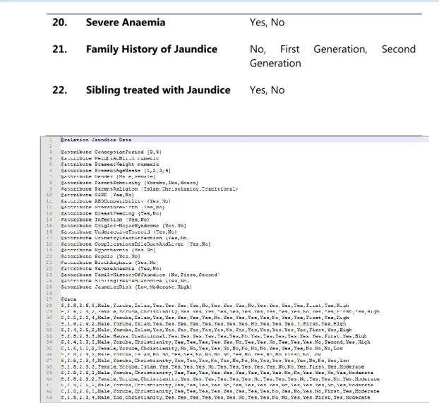
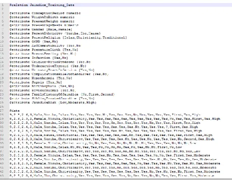
The data was then transformed into the attribute file format (.raff) for the purpose of the development of the predictive model for infertility risk using the simulation environment. Figure 1 shows a screenshot of the format of the. raff used for model development in the Waikato Environment for Knowledge Analysis (WEKA) – a light-weight java application composed of a suite of supervised and unsupervised machine learning tools.
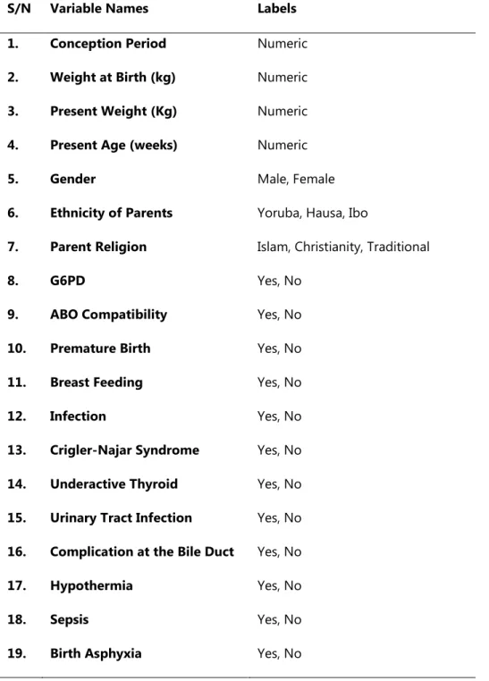
Table 1: Identified variables for determining Jaundice
S/N Variable Names Labels
1. Conception Period Numeric
2. Weight at Birth (kg) Numeric
3. Present Weight (Kg) Numeric
4. Present Age (weeks) Numeric
5. Gender Male, Female
6. Ethnicity of Parents Yoruba, Hausa, Ibo
7. Parent Religion Islam, Christianity, Traditional
8. G6PD Yes, No
9. ABO Compatibility Yes, No
10. Premature Birth Yes, No
11. Breast Feeding Yes, No
12. Infection Yes, No
13. Crigler-Najar Syndrome Yes, No 14. Underactive Thyroid Yes, No 15. Urinary Tract Infection Yes, No 16. Complication at the Bile Duct Yes, No
17. Hypothermia Yes, No
18. Sepsis Yes, No
20. Severe Anaemia Yes, No
21. Family History of Jaundice No, First Generation, Second Generation
22. Sibling treated with Jaundice Yes, No
Figure 1: arff file containing identified attributes The arff file is composed of three parts, namely:
a. The relation name section which contains the tag @relation Jaundice_Data, used to identify the name of the relation (or file) that contains the data needed for simulation. This section is located at the first line of the file and the tag ‘name’ following @relation must always be the same as the file name else the file loader of the simulation environment will cease to open the file. This section is followed in the next line by the attribute names section;
b. The attribute names section which contains the tag @attribute attribute_name label was used to identify the attributes that describe the dataset stored in the .arff file needed for simulation. Each attribute name alongside its labels is stated following the @relation tag on each line. The label can be a set of values inserted between brackets or a descriptor (e.g. date, numeric etc.). The last attribute is identified as the target class (risk of jaundice) while the previous attributes are the risk factors for the risk of jaundice. This section is followed in the next line by the data section; and
c. The data section which contains the tag @data followed in the next line by the values of the attributes for each record of the risk of jaundice separated by a comma. Each value was listed on a row for each record in the same order as the attributes were listed in the attribute names section. The values inserted into each record must be the same values defined in each respective attribute; if there is an error in spelling or a label not defined is inserted then the file loader of the simulation environment will fail to load the file.
The dataset collected for the purpose of the development of the predictive model for the diagnosis of jaundice was stored in .arff in the name Jaundice_Data.arff while the number of attributes listed in the attribute section were 23 including the target attribute. Following this, the values of the risk factors for the record of the 49 neonates considered for this study was provided.
3.4 Formulation of the Predictive Model for Classification of Risk of jaundice
Systems that construct classifiers are one of the commonly used tools in data mining. Such systems take as input a collection of cases, each belonging to one of a small number of classes and described by its values for a fixed set of attributes, and output a classifier that can accurately predict the class to which a new case belongs. Supervised machine learning algorithms make it possible to assign a set of records (jaundice risk indicators) to a target classes – the diagnosis of jaundice (Low, Moderate, High).
Supervised machine learning algorithms are Black-boxed models, thus it is not possible to give an exact description of the mathematical relationship existing among the independent variables (input variables) with respect to the target variable (output variable – risk of jaundice). Cost functions are used by supervised machine learning algorithms to estimate the error in prediction during the training of data for model development. Although, the decision trees algorithm is a white-boxed model owing to its ability of been interpreted as a tree-structure.
For any supervised machine learning algorithm proposed for the formulation of a predictive model, a mapping function can be used to easily express the general expression for the formulation of the predictive model for the classification of risk of jaundice – this is as a result that most machine learning algorithms are black-box models which use evaluators and not power series/polynomial equations. The historical dataset S which consists of the records of neonates containing fields representing the set of classification factors (i number of input variables for j neonates), 𝑋𝑖𝑗 alongside the respective target variable (risk of jaundice) represented by the variable 𝑌𝑗 – the risk of jaundice for the jth individual in the j records of data collected from the hospital selected for the study. Equation 1 shows the mapping function that describes the relationship between the classification factors and the target class – classification of risk of jaundice.
φ: X → Y (1) defined as: φ(X) = Y
The equation shows the relationship between the set of classification factors represented by a vector, X
consisting of the values of i variables and the label Y which defines the risk of jaundice – Yes and No for each neonate as expressed in equation 2. Assuming the values of the set of variable for a neonate is represented as 𝑋 = {𝑋1, 𝑋2, 𝑋3, . . . , 𝑋𝑖} where 𝑋𝑖 is the value of each variable, i = 1 to i; then the mapping 𝜑 used to represent the predictive model for neonate performance maps the variables of each individual to their respective risk of jaundice according to equation 2.
𝜑(𝑋) = {ModerateLow
High (2)
The developed predictive model for the risk of jaundice was used to propose a set of rules that can be used to determine the risk of jaundice directly just by observing the value of the variables identified by the model and the succession of events. In the following section, the machine learning algorithms used in formulating the predictive model for the risk of jaundice are presented.
Naïve Bayes’ Classifier
Naive Bayes’ Classifier is a probabilistic model based on Bayes’ theorem. It is defined as a statistical classifier. It is one of the frequently used methods for supervised learning. It provides an efficient way of handling any number of attributes or classes which is purely based on probabilistic theory. Bayesian classification provides practical learning algorithms and prior knowledge on observed data.
Let 𝑋𝑖𝑗 be a dataset sample containing records (or instances) of i number of risks factors (attributes/features) alongside their respective diagnosis of jaundice, C (target class) collected for j number of records/neonates and 𝐻𝑘= {𝐻1= 𝐿𝑜𝑤, 𝐻2= 𝑀𝑂𝑑𝑒𝑟𝑎𝑡𝑒, 𝐻3= 𝐻𝑖𝑔ℎ} be a hypothesis that 𝑋𝑖𝑗 belongs to class C. For the classification of the risk of infertility given the values of the risk factor of the jth record, Naïve Bayes’ classification required the determination of the following:
• 𝑃(𝐻𝑘|𝑋𝑖𝑗) – Posteriori probability: is the probability that the hypothesis, 𝐻𝑘 holds given the observed data sample 𝑋𝑖𝑗 for 1 ≤ 𝑘 ≤ 3.
• 𝑃(𝐻𝑘) - Prior probability: is the initial probability of the target class 1 ≤ 𝑘 ≤ 3;
• 𝑃(𝑋𝑖𝑗) is the probability that the sample data is observed for each risk factor (or attribute), i; and
• 𝑃(|𝑋𝑖𝑗|𝐻𝑘) is the probability of observing the sample’s attribute, 𝑋𝑖 given that the hypothesis holds in the training data 𝑋𝑖𝑗.
Therefore, the posteriori probability of an hypothesis 𝐻𝑘 is defined according to Bayes’ theorem as follows:
𝑃(𝐻𝑘|𝑋𝑖𝑗) =
∏𝑛𝑖=1𝑃(𝑋𝑖𝑗|𝐻𝑘)𝑃(𝑋𝑖)
𝑃(𝐻𝑘) 𝑓𝑜𝑟 𝑘 = 1,2,3 (3) Hence, the risk of jaundice for a record is thus:
𝑚𝑎𝑥. [𝑃(𝐻1|𝑋𝑖𝑗), 𝑃(𝐻2|𝑋𝑖𝑗), 𝑃(𝐻3|𝑋𝑖𝑗)] (4) Multi-layer Perceptron
An artificial neural network (ANN) is an interconnected group of nodes, akin to the vast network of neurons in a human brain. In machine learning and cognitive science, ANNs are a family of statistical learning models inspired by biological neural networks and are used to estimate or approximate functions that depend on a large number of inputs and are generally unknown. ANNs are generally presented as systems of interconnected neurons which send messages to each other such that each connection have numeric weights that can be tuned based on experience, making neural nets adaptive to inputs and capable of learning.
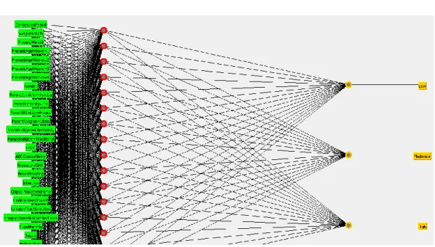
The word network refers to the inter-connections between the neurons in the different layers of each system. The first layer has input neurons (CML survival indicators) which send data via synapses to the middle layer of neurons, and then via more synapses to the third layer of output neurons (see Figure 2). The synapses store parameters called weights that manipulate the data stored in the calculations. An ANN is typically defined by three (3) types of parameters, namely:
i.Interconnection pattern between the different layers of neurons; ii.Learning process for updating the weights of the interconnections; and
Multi-layer networks use a variety of learning techniques, the most popular been back-propagation. Back-propagation, an abbreviation for backward propagation of errors, is a common method of training artificial neural networks used in conjunction with an optimization method such as gradient descent. The method calculates the gradient of a loss function with respect to all the weights in the network. The gradient is fed to the optimization method which in turn uses it to update the weights, in an attempt to minimize the loss function. It is a generalization of the delta rule to multi-layered feed-forward networks, made possible by using the chain rule to iteratively compute gradients for each layer. Back-propagation requires that the activation function used by the artificial neurons be differentiable
The back-propagation learning algorithm can be divided into two phases: propagation and weight update. • Phase 1 – Propagation: each propagation involves the following steps:
o Forward propagation of training pattern’s input through the neural network in order to
generate the propagation’s output activations; and
o Backward propagation of the propagation’s output activations through the neural
network using the training pattern target in order to generate deltas of all output and hidden neurons.
• Phase 2 – Weight update: for each weight-synapse, hence the following:
o Multiply its output delta and input activation to get the gradient of the weight; and o Subtract a ratio (percentage) of the gradient from the weight.
Figure 2: Multi-layer perceptron architecture for risk of jaundice
In this study, the input neurons were represented by each jaundice risk indicator variables determined by Xi = {X1, X2, X3 ….Xi} where i is the number of variables (input neurons). The effect of the synaptic weights, Wi on each input neuron at layer j is represented by the expression:
Equation (10) is sent to the activation function (sigmoid/logistic function) was applied in order to limit the output to a threshold [-1, +1], thus:
𝑉𝑗= 𝜑(𝑧) = 1
1 + 𝑒−𝑧𝑗 (6)
The measure of discrepancy between the expected output (p) and the actual output (y) was made using the squared error measure (E):
𝐸 = (𝑝 − 𝑦)2 (7)
Recall however, that the output (p) of a neuron depends on the weighted sum of all its inputs as indicated in equation (5); implying that the error (E) also depends on the incoming weights of the neuron which needs to be changed in the network to enable learning. The back-propagation algorithm was used to find the set of weights that minimizes the error. In this study, the gradient descent algorithm was applied in order to minimize the error and hence find the optimal weights that satisfy the problem. Since back-propagation uses the gradient descent method, there was a need to calculate the derivative of the squared error function with respect to the weights of the network. Hence, the squared error function is now redefined as (the ½ is required to cancel the exponent of 2 when differentiating):
𝐸 = 1
2(𝑝 − 𝑦)2 (8) For each neuron, j its output Oj is defined as:
𝑂𝑗= 𝜑(𝑛𝑒𝑡𝑗) = 𝜑 (∑ 𝑤𝑖𝑗𝑥𝑖 𝑛
𝑘=1
) (9)
The input 𝑛𝑒𝑡𝑗 to a neuron is the weighted sum of outputs 𝑂𝑖of the previous neurons. The number of input neurons is n and the variable 𝑤𝑖𝑗 denotes the weight between neurons I and j. The activation function 𝜑 is in general non-linear and differentiable, thus, the derivative of the equation (6) is:
𝜕𝜑
𝜕𝑧 = 𝜑(1 − 𝜑)(10)
The partial derivative of the error (E) with respect to a weight 𝑤𝑖𝑗was done using the chain rule twice as follows: 𝜕𝐸 𝜕𝑤𝑖𝑗 = 𝜕𝐸 𝜕𝑂𝑗 𝜕𝑂𝑗 𝜕𝑛𝑒𝑡𝑗 𝜕𝑛𝑒𝑡𝑗 𝜕𝑤𝑖𝑗 (11) The last term on the left hand side can be calculated from equation (9), thus:
𝜕𝑛𝑒𝑡𝑗 𝜕𝑤𝑖𝑗 = 𝜕 𝜕𝑤𝑖𝑗(∑ 𝑤𝑖𝑗𝑥𝑖 𝑛 𝑘=1 ) = 𝑥𝑖(12)
The derivative of the output of neuron j with respect to its input is the partial derivative of the activation function (logistic function) shown in equation (10):
𝜕𝑂𝑗 𝜕𝑛𝑒𝑡𝑗=
𝜕
𝜕𝑛𝑒𝑡𝑗𝜑(𝑛𝑒𝑡𝑗) = 𝜑(𝑛𝑒𝑡𝑗) (1 − φ(netj)) (13)
The first term is evaluated by differentiating the error function in equation (9) with respect to y, so if y is in the outer layer such that y =Oj, then:
∂E ∂Oj= ∂E ∂y= ∂ ∂y 1 2(p − y)2= y − p (14)
However, if j when in an arbitrary inner layer of the network, finding the derivative E with respect to Ojwas less obvious. Considering E as a function of the inputs of all neurons, i receiving input from neuron j and taking the total derivative with respect toOj, a recursive expression for the derivative was obtained:
∂E ∂Oj = ∑ ( ∂E ∂netl ∂netl ∂Oj ) = lϵL ∑ (∂E ∂Ol ∂Ol ∂netlwjl) lϵL (15)
Thus, the derivative with respect to Ojcan be calculated if all the derivatives with respect to the outputs 𝑂𝑗of the next layer – the one closer to the output neuron – are known. By putting them all together:
∂E ∂wij= δjxi (16) With: δj= ∂E ∂Oj ∂Oj ∂netj= {
(Oj− pj)φ(netj) (1 − φ(netj)) if j is an output neuron, (∑ δjwjl)φ(netj) (1 − φ(netj)) if j is an inner neuron
lϵL
Therefore, in order to update the weight wijusing gradient descent, one must choose a learning rate, 𝛼. The change in weight, which was added to the old weight, is equal to the product of the learning rate and the gradient, multiplied by -1:
∆wij= −α ∂E
∂wij (17)
Equation (17) was used by the back-propagation algorithm to adjust the value of the synaptic weights attached to the inputs at each neuron in equation (5) with respect to the inner layer of the multi-layer perceptron classifier. 3.5 Model Simulation Process and Environment
Following the identification of the supervised machine learning algorithms that was needed for the formulation of the predictive model for the classification of risk of jaundice, the simulation of the predictive model was performed using the data collected which consisted of neonates records containing information about the input variables and their respective value of risk of jaundice collected from the hospital located in south-western Nigeria. The Waikato Environment for Knowledge Analysis (WEKA) software – a suite of machine learning algorithms was used as the simulation environment for the development of the predictive model.
The dataset collected was divided into two parts: training and testing data – the training data was used to formulate the model while the test data was used to validate the model. The process of training and testing predictive model according to literature is a very difficult experience especially with the various available validation procedures. For this classification problem, it was natural to measure a classifier’s performance in terms of the error rate. The classifier predicted the class of each instance – the neonate’s record containing values for each variable for risk of jaundice: if it is correct, that is counted as a success; if not, it is an error. The error rate being the proportion of errors made over a whole set of instances, and thus measured the overall performance of the classifier. The error rate on the training data set was not likely to be a good indicator of future performance; because the DT classifiers were been learned from the very same training data.
In order to predict the performance of a classifier on new data, there was the need to assess the error rate of the predictive model on a dataset that played no part in the formation of the classifier. This independent dataset was called the test dataset – which was a representative sample of the underlying problem as was the training data. It was important that the test dataset was not used in any way to create the classifier since the machine learning classifiers involve two stages: one to come up with a basic structure of the predictive model and the second to optimize parameters involved in that structure.
10-fold cross validation technique
The process of leaving a part of a whole dataset as testing data while the rest is used for training the model is called the holdout method. The challenge here is the need to be able to find a good classifier by using as much of the whole historical data as possible for training; to obtain a good error estimate and use as much as possible for model testing. It is a common trend to holdout one-third of the whole historical dataset for testing and the remaining two-thirds for training.
For this study the cross-validation procedure was employed, which involved dividing the whole datasets into a number of folds (or partitions) of the data. Each partition was selected for testing with the remaining k – 1 partitions used for training; the next partition was used for testing with the remaining k – 1 partitions (including the first partition used or testing) used for training until all k partitions had been selected for testing. The error rate recorded from each process was added up with the mean the mean error rate recorded. The process used in this study was the stratified 10-fold cross validation method which involves splitting the whole dataset into ten partitions.
Simulation environment
Weka is open source software under the GNU General Public License. The system was developed at the University of Waikato in New Zealand. Weka stands for the Waikato Environment for Knowledge Analysis. The software is freely available at http://www.cs.waikato.ac.nz/ml/weka. The system was written using object-oriented language, Java.
There are several different levels at which Weka can be used. Weka provides implantations of state-of-the-art data mining and machine learning algorithms. Weka contains modules for data pre-processing, classification, clustering and association rule extraction for market basket analysis. The main features of Weka include:
a. 49 data preprocessing tools;
b. 76 classification/regression algorithms; c. 8 clustering algorithms;
d. 15 attribute/subset evaluators + 10 search algorithms for feature selection; e. 3 algorithms for finding association rules; and
f. 3 graphical user interfaces, namely: i.The Explorer for exploratory data analysis;
ii.The Experimenter for experimental environment; and
Before subjecting the historical datasets containing the values of the variables alongside the risk of jaundice for each neonate’s record in the original dataset; there was the need of storing the dataset according to the default format for data representation needed for data mining tasks on the Weka environment. The default file type is called the attribute relation file format (.arff). the arff file type stores three category of data: the first defining the title of the relation, the second defining the relation’s attributes alongside their respective labels and the third defining the relations data followed for the values of each attributes for each record. Also, data can be read from comma separated values (.csv) format and from databases using Object-Database Connectivity (ODBC).
3.6 Performance Evaluation of Model Validation Process
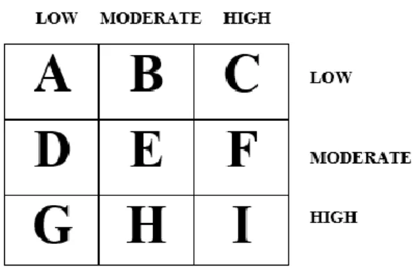
During the course of evaluating the predictive model, a number of metrics were used to quantify the model’s performance. In order to determine these metrics, four parameters must be identified from the results of predictions made by the classifier during model testing. These are: true positive (TP), true negative (TN), false positive (FP) and false negative (FP). True positives are the correct prediction of positive cases, true negatives are the correct prediction of negative cases, and false positives are the negative cases predicted as positives while false negatives are positive cases predicted as negatives. These results are presented on confusion matrix – for this study the confusion matrix is a 3 x 3 matrix table owing to the three (3) labels of the output class (see Figure 3).
Correct classifications were plotted along the diagonal from the north-west position for low predicted as low (A), moderate predicted as moderate (E) and high predicted as high (I) on the south-east corner (all called true positives and negatives). The incorrect classifications were plotted in the remaining cells of the confusion matrix
Figure 3: Diagram of a Confusion Matrix
(also called false positives and negatives). Also, the actual low cases are A+B+C, actual moderate cases are D+E+F while actual high cases are G+H+I and the predicted low are A+D+G, moderate are B+E+H and predicted high are C+F+I.The developed model was validated a number of performance metrics based on the values of A
– I in the confusion matrix for each predictive model. They are presented as follows. a. Accuracy: the total number of correct classifications
𝐴𝑐𝑐𝑢𝑟𝑎𝑐𝑦 = 𝐴 + 𝐸 + 𝐼
𝑡𝑜𝑡𝑎𝑙_𝑐𝑎𝑠𝑒𝑠 (18)
b. True positive rate (recall/sensitivity): the proportion of actual cases correctly classified.
𝑇𝑃𝑙𝑜𝑤 = 𝐴
𝑇𝑃𝑚𝑜𝑑𝑒𝑟𝑎𝑡𝑒= 𝐸
𝐷 + 𝐸 + 𝐹 (19𝑏) 𝑇𝑃ℎ𝑖𝑔ℎ= 𝐼
𝐺 + 𝐻 + 𝐼 (19𝑐)
c. False positive (false alarm/1-specificity): the proportion of negative cases incorrectly classified as positive. 𝐹𝑃𝑙𝑜𝑤 = 𝐷 + 𝐺 𝑎𝑐𝑡𝑢𝑎𝑙𝑚𝑜𝑑𝑒𝑟𝑎𝑡𝑒+ 𝑎𝑐𝑡𝑢𝑎𝑙ℎ𝑖𝑔ℎ (20𝑎) 𝐹𝑃𝑚𝑜𝑑𝑒𝑟𝑎𝑡𝑒= 𝐵 + 𝐻 𝑎𝑐𝑡𝑢𝑎𝑙𝑙𝑜𝑤+ 𝑎𝑐𝑡𝑢𝑎𝑙ℎ𝑖𝑔ℎ (20𝑏) 𝐹𝑃ℎ𝑖𝑔ℎ= 𝐶 + 𝐹 𝑎𝑐𝑡𝑢𝑎𝑙𝑙𝑜𝑤+ 𝑎𝑐𝑡𝑢𝑎𝑙𝑚𝑜𝑑𝑒𝑟𝑎𝑡𝑒 (20𝑐) d. Precision: the proportion of predictions that are correct
𝑃𝑟𝑒𝑐𝑖𝑠𝑖𝑜𝑛𝑙𝑜𝑤= 𝐴 𝐴 + 𝐷 + 𝐺 (21𝑎) 𝑃𝑟𝑒𝑐𝑖𝑠𝑖𝑜𝑛𝑚𝑜𝑑𝑒𝑟𝑎𝑡𝑒= 𝐸 𝐵 + 𝐸 + 𝐻 (21𝑏) 𝑃𝑟𝑒𝑐𝑖𝑠𝑖𝑜𝑛ℎ𝑖𝑔ℎ= 𝐼 𝐶 + 𝐹 + 𝐼 (22)
Using the aforementioned performance metrics, the performance of the predictive model for the classification of student’s performance can be evaluated by validation using a historical dataset collected based on the information provided in the questionnaire. The TP rate and precision lie within the interval [0, 1], accuracy within the interval of [0, 100]% while the FP rate lies within an interval of [0, 1]. The closer the accuracy is to 100% the better the model, the closer the value of the TP rate and precision is to 1 the better while the closer the value of FP rate is to 0 the better. Therefore, the evaluation of an effective model has a high TP/Precision rates and a low FP rate.
4. Results
In this section of the study, the results of the methodological approach described earlier are discussed. A thorough investigation into the analysis of the description of the dataset collected was initially performed in order to understand the distribution of the values of the variable for each risk of jaundice among the neonates selected for this study using the minimum and maximum values, and the mean and standard deviation of the data distribution. The numeric variables identified and collected for this study were also discretized into nominal values so as to reduce the computational complexity associated with numeric variable. Following this, the results of the model formulation and simulation process for the development of the predictive model for the classification risk of jaundice was presented.
4.1 Result of the Data Identified and Collected
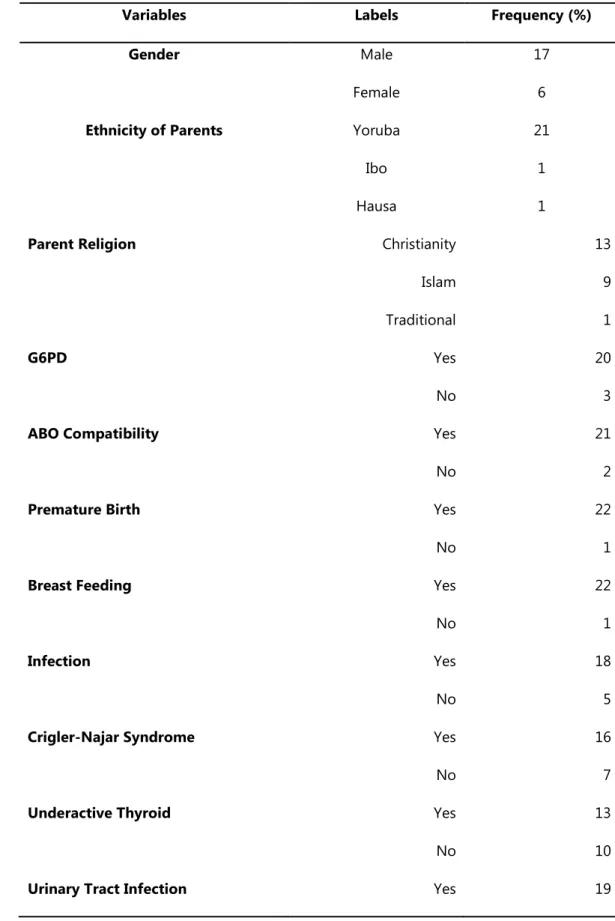
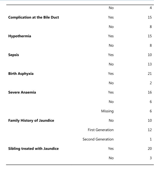
The analysis of the data containing information about the attributes for the 49 neonates are shown in Tables 2 and 3. Table 2 shows the description of the nominal variables while Table 3 shows the distribution of the numeric variables. From the description shown in Table 2, there were more female than male respondents owing for a ratio of 1:1.33 for men to women. The number of records diagnosed of jaundice consisted of 67.3% of the
dataset while the remaining consisting of those without jaundice. Chest pain and exam had missing values of 7 and 6 respectively representing about 14.3% and 12.2% of the data values for each variable respectively.
Table 2: Description of the nominal variables in the dataset
Variables Labels Frequency (%)
Gender Male
Female
17 6
Ethnicity of Parents Yoruba
Ibo Hausa
21 1 1
Parent Religion Christianity
Islam Traditional 13 9 1 G6PD Yes No 20 3
ABO Compatibility Yes
No
21 2
Premature Birth Yes
No
22 1
Breast Feeding Yes
No 22 1 Infection Yes No 18 5
Crigler-Najar Syndrome Yes
No
16 7
Underactive Thyroid Yes
No
13 10
No 4
Complication at the Bile Duct Yes
No 15 8 Hypothermia Yes No 15 8 Sepsis Yes No 10 13
Birth Asphyxia Yes
No
21 2
Severe Anaemia Yes
No Missing
16 6 6
Family History of Jaundice No
First Generation Second Generation
10 12 1
Sibling treated with Jaundice Yes
No
20 3
Table 3: Description of the numeric variables in the dataset
Variables Minimum Maximum Mean Standard
Deviation
Conception Period (months) 8 9 8.39 0.499
Weight at Birth (Kg) 1.60 2.90 2.56 0.261
Present Weight (Kg) 1.50 2.90 2.38 0.250
Present age (weeks) 2 4 2.74 0.689
From the description shown in Table 3, the analysis of the numeric datasets is presented showing the values of the minimum, maximum, mean and standard deviation of each variable presented in the dataset. Following the
description of the numeric dataset, the numeric dataset was discretized into nominal datasets by creating intervals to which classes were defined. Figure 4 shows a diagram of the arff file for the new training data stored in the file Jaundice_training_data. arff.
4.2 Model Formulation and Simulation
Two different supervised machine learning algorithms were used to formulate the predictive model for the diagnosis of jaundice, namely: Naïve Bayes’ and decision trees classifiers. They were used to train the development of the prediction model using the dataset containing 49 neonates’ risk factor records. The simulation of the prediction models was done using the Waikato Environment for Knowledge Analysis (WEKA). The Naïve Bayes’ algorithm was implemented using the Naïve Bayes classifier available in the Bayes classifiers while the multi-layer perceptron algorithm was implemented using the Multilayer Perceptron classifier available in the function’s classifier both available on the WEKA Explorer environment for classification tools. The models were trained using the 10-fold cross validation method which splits the dataset into 10 subsets of data – while 9 parts are used for training the remaining one is used for testing; this process is repeated until the remaining 9 parts take their turn for testing the model.
Figure 4: arff file containing identified attributes after data pre-processing Results of the Naïve Bayes’ classifier
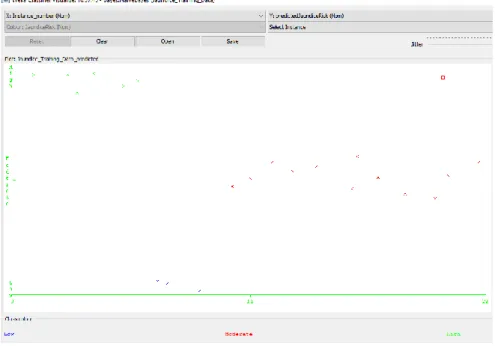
Following the simulation of the predictive model for classification of risk of jaundice using the Naïve Bayes’ classifier, the evaluation of the performance of the model following validation using the 10-fold cross validation method was recorded. Figure 5 shows the screenshot of the results of the predictions made by the Naïve Bayes’ classifier algorithm for the 23 instances of data collected from the neonates considered for this study. The figures show the correct and incorrect classifications made by the algorithm while Figure 6 shows the graphical plot of the predictions made by the Naïve Bayes’ classifier algorithm on the dataset. In figure 6, each class of risk of jaundice is represented using a specific colour and each correct classification is represented with a star while each misclassification is represented as a square.
The results presented in figure 6 was used to evaluate the performance of the Naïve Bayes’ classifier algorithm and thus, the confusion matrix determined. Figure 7 shows the confusion matrix that was used to interpret the results of the true positive and negative alongside the false positive and negatives of the validation results. The
confusion matrix shown in figure 7 was used to evaluate the performance of the predictive model for classification of risk of jaundice.
Based on the results presented in the confusion matrix with the Naïve Bayes’ classifier used to train the predictive model developed using the training data via the 10-fold cross validation method, it was discovered that there were 21 (91.30%) correct classifications (3 for Low, 12 for Moderate and 6 for High – along the diagonal) and 2 (8.70%) incorrect classifications 1moderate for high and 1high for moderate as shown in figure 7. Hence, the predictive model for the risk of infertility using the Naïve Bayes’ classifier showed an accuracy of 91.30%.
Figure 5: Screenshot of Naïve Bayes’ classifier results on dataset
Figure 7: Confusion matrix for the result of Naïve Bayes’ classifier
From the information provided by the confusion matrix, it was discovered that all of the 3 low cases were correctly classified; out of the 13 moderate cases, 12 were correctly classified while 1 was misclassified as high and out of the 7 high cases, 6 were correctly classified while 1 was misclassified as moderate.
Table 4 shows the results of the evaluation of the performance of the Naïve Bayes’ classifier using the metrics. Based on the results presented for the naive Bayes’ classifier, the TP rate of the model was better for the low cases than for the moderate and high cases thus the model has the ability to predict the low better than the other cases (an average of 92.7% of actual cases); the FP rate for the low cases were also better than that of the moderate and high cases although the high cases was better than the moderate cases (an average of 5.4% of the actual cases) while for the precision, the model performed very well in predicting the Low cases than that of the moderate and high cases since most of the predictions made by the model were correct (with an average of 92.7% of the predicted cases). The results further showed that the model developed using the Naïve Bayes’ classifier misclassified a proportion of moderate cases as high cases and vice versa.
Results of the Multi-Layer Perceptron
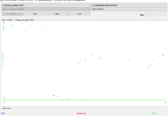
Following the simulation of the predictive model for classification of risk of jaundice using the multi-layer perceptron, the evaluation of the performance of the model following validation using the 10-fold cross validation method was recorded. Figure 8 shows the screenshot of the results of the predictions made by the multi-layer perceptron algorithm for the 23 instances of data collected from the neonates considered for this study. The figures show the correct and incorrect classifications made by the algorithm while Figure 9 shows the graphical plot of the predictions made by the multi-layer perceptron algorithm on the dataset. In figure 9, each class of risk of jaundice is represented using a specific colour and each correct classification is represented with a star while each misclassification is represented as a square.
Table 4: Performance evaluation of the results of the Naïve Bayes’ classifier
Class TP rate FP rate Precision Area under the ROC
Low 1.000 0.000 1.000 1.000
Moderate 0.923 0.100 0.923 0.977
High 0.857 0.063 0.857 0.973
Figure 8: Screenshot of multi-layer perceptron results on dataset
Figure 9: Screenshot of correct and incorrect classifications made by multi-layer perceptron
The results presented in figure 9 was used to evaluate the performance of the multi-layer perceptron algorithm and thus, the confusion matrix determined. Figure 10 shows the confusion matrix that was used to interpret the results of the true positive and negative alongside the false positive and negatives of the validation results. The
confusion matrix shown in figure 10 was used to evaluate the performance of the predictive model for classification of risk of jaundice.
Based on the results presented in the confusion matrix with the multi-layer perceptron used to train the predictive model developed using the training data via the 10-fold cross validation method, it was discovered that there were 23 (100%) correct classifications (3 for low, 13 for moderate and 7 for high cases – along the diagonal) and no (0%) incorrect classifications as shown in figure 10. Hence, the predictive model for the risk of infertility using the multi-layer perceptron showed an accuracy of 100%.
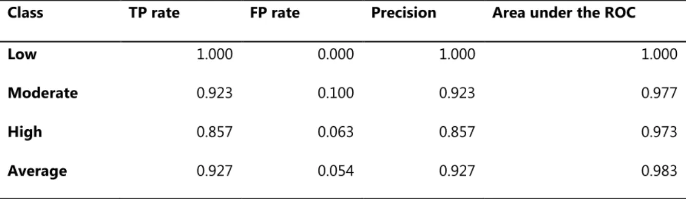
Table 5 shows the results of the evaluation of the performance of the multi-layer perceptron using the metrics. Based on the results presented for the multi-layer perceptron, the TP rate, FP rate and the precision all had values of 1 while the FP rate had a value of 0 for both the Yes and No cases. Therefore, the predictive model developed using the multi-layer perceptron was able to properly distinguish between the Low, moderate and High cases available in the dataset presented for this study.
Figure 10: Confusion matrix for the result of multi-layer perceptron Table 5: Performance evaluation of the results of the multi-layer perceptron
Class TP rate FP rate Precision Area under the
ROC Low 1.000 0.000 1.000 1.000 Moderate 1.000 0.000 1.000 1.000 High 1.000 0.000 1.000 1.000 Average 1.000 0.000 1.000 1.000 4.4 Discussion of results
The result of the performance evaluation of the machine learning algorithms are presented in Table 6 which presents the average values of each performance evaluation metrics considered for this study. For the Naïve Bayes’ classifier algorithm based on the results presented in the confusion matrix presented in figure 7. The results showed that the TP rate which gave a description of the proportion of actual cases that was correctly predicted was 0.927 which implied that 92.7% of the actual cases were correctly predicted; the FP rate which
gave a description of the proportion of actual cases misclassified was 0.054 which implied that 5.4% of actual cases were misclassified while the precision which gave a description of the proportion of predictions that were correctly classified was 0.927 which implied that 92.7% of the predictions made by the classifier were correct. For the multi-layer perceptron algorithm based on the results presented in the confusion matrix presented in figure 10. The results showed that the TP rate which gave a description of the proportion of actual cases that was correctly predicted was 1 which implied that 100% of the actual cases were correctly predicted; the FP rate which gave a description of the proportion of actual cases misclassified was 0 which implied that 0% of actual cases were misclassified while the precision which gave a description of the proportion of predictions that were correctly classified was 1 which implied that 100% of the predictions made by the classifier were correct. In general, multi-layer perceptron algorithm were able to classify the performance of students by graduation better than the Naïve Bayes’ classifier algorithm. The multi-layer perceptron algorithm was able to accurately classify all cases of jaundice with a value of 100%.
Table 6: Summary of the results of performance evaluation for the machine learning algorithms selected Machine Learning
Algorithm Used
PERFORMANCE EVALUATION METRICS Correct Classification (out of 23) Accuracy (%) TP rate (recall/sensi tivity) FP rate (false positive) Precision Naïve Bayes’ Classifier 21 91.3 0.927 0.054 0.927 Multi-Layer Perceptron 23 100.0 1.000 0.000 1.000 5. Conclusion
This study will contribute to knowledge by using decision trees algorithm for the identification of relevant features for the risk of jaundice thereby improving the decision-making process involved in the early detection of the risk of jaundice.
In this paper, the development of a predictive model for predicting the diagnoses of jaundice given the values of risk factors was developed using dataset collected from neonates in a hospital in the south-western part of Nigeria. 10 variables were identified by the medical expert to be necessary in predicting jaundice in neonates for which a dataset containing information of 23 neonates alongside their respective jaundice diagnosis (Low, Moderate and High) was also provided with 22 attributes following the identification of the required variables. After the process of data collection and pre-processing, two supervised machine learning algorithms were used to develop the predictive model for the diagnosis of jaundice using the historical dataset from which the training and testing dataset was collected. The 10-fold cross validation method was used to train the predictive model developed using the machine learning algorithms and the performance of the models evaluated. The multi-layer perceptron algorithm proved to be an effective algorithm for predicting the diagnosis of jaundice in Nigerian neonates.
It is recommended that the be integrated into existing Health Information System (HIS) which captures and manages clinical information which can be fed to the jaundice predictive model thus improving the decisions
affecting the neonate’s outcome and the real-time assessment of clinical information affecting neonate’s risk of jaundice.
References
1. Agbelusi, O. (2014). Development of a predictive model for survival of HIV/AIDS patients in South-western Nigeria, Unpublished MPhil Thesis, Obafemi Awolowo University, Ile-Ife, Nigeria.
2. Ahmed, H., Yukubu, A.M. and Hendrickse, R.G. (1995). Neonatal jaundice in Zaria, Nigeria--a second prospective study. West Africa Journal of Medicine 14(1):15- 23.
3. American Academy of Pediatrics Subcommittee on Hyperbilirubinaemia (2004). Management of Hyperbilirubinaemia in the newborn infant 35 or more weeks of gestation. Pediatrics 114(1): 297-316. 4. Balogun, J. A., Egejuru, N. C/ and Idowu P. A. (2018). Comparative Analysis of Predictive Models for the
Likelihood of Infertility in Women Using Supervised Machine Learning Techniques Computer Reviews Journal 2(1): 313-330 ISSN: 2581-6640
5. Behrman, R.E., Kliegman, R.M. and Jenson, H.B., editors. Nelson Textbook of Pediatrics. 16th edition. Philadelphia: Saunders: 511- 528.
6. Bilgen, H., Ozek, E., Unver, T., Biyikli, N., Alpay, H. and Cebeci, D. (2006). Urinary tract infection and hyperbilirubinaemia. Turkish Journal of Pediatric 48(1):51- 55.
7. Chen, H.Y., Chuang, C.H., Yang, Y.J. and Wu, T.P. (2011). Exploring the risk factors of preterm birth using data mining. Expert Syst Appl 38(5):5384– 5387.
8. Coleman, R. (2011). Newborn Jaundice and Vitamin D. Retrieved from
http://www.livestrong.com/article/532575-newbornjaundice-vitamin-d/#ixzz2a3FMIuBl on March 21,
2017.
9. Delen, D., Walker, G. and Kadam, A. (2005). Predicting breast cancer survivability: a comparison of three data mining methods. Artif Intell Med 34(2):113–127.
10. Dennery, P.A., Seidman, D.S. and Stevenson, D.K. (2001). Neonatal hyperbilirubinaemia. New Engl J Med 344:581 – 590.
11. Effiong, C.E., Aimaku, V.E., Bienzle, U., Oyedeji, G.A. and Ikpe, D.E. (1975). Neonatal Jaundice in Ibadan, incidence and aetiologic factors in babies born in Hospital. Journal of the National Medical Association 67(3): 1 – 13
12. Egube, B.A., Ofili, A.N. and Onakewhor, J.U. (2013). Neonatal Jaundice and its management: Knowledge, attitude, and practice among expectant mothers attending antenatal clinic at University of Benin teaching Hospital, Benin City, Nigeria. Nigerian Journal of Clinical Practice 16(2): 188 – 194.
13. Eneh, A.U. and Ugwu, R.O. (2009). Perception of neonatal jaundice among women attending children outpatient and immunization clinics in Port Harcourt. Niger. J. Clin. Pract. 12(2): 187-191.
14. Ezechukwu, C.C., Ugochukwu, E.F., Egbuonu, I. and Chukwuka, J.O. (2004). Risk factors from neonatal mortality in regional tertiary hospital in Nigeria. Niger J Clin Pract 7:50- 52.
15. Ferreira, D., Oliveira, A. and Freitas, A. (2012). Applying data mining techniques to improve diagnosis in neonatal jaundice. BMC Medical Informatics and Decision Making 12(143): 1 – 6.
16. Hagar, F.S., Taha, E.T. and Mervat, M.M. (2012). Applying Data Mining Techniques for the Optimal Usage of Neonatal Incubator. International Journal of Computer Applications 52(3): 11 – 20.
17. Han, J. and Kamber, M. (2006). Data mining concepts and techniques (2nd edition). Morgan Kaufmann publisher, New York, USA.
18. Haque, K.M. and Rahman, M. (2000). An unusual case of ABO-Haemolytic Disease of the Newborn.
Bangladesh Med. Res. Counc. Bull. 16(3): 105-108
19. Ho, N.K. (2002). Neonatal jaundice in Asia. Baillieres Clin. Haematol. 5(1): 131-142.
20. Idowu, P.A., Aladekomo, T.A., Williams, K.O. and Balogun, J.A. (2015). Predictive model for likelihood of Sickle cell aneamia (SCA) among pediatric patients using fuzzy logic. Transactions in networks and communications 31(1): 31 – 44.
21. Ipek, I.O. and Bozayakut, A. (2008). Clinically significant neonatal hyperbilirubinaemia: an analysis of 546 cases in Istanbul. J. Trop. Pediatr., 54: 212-213.
22. Kantardzic, M. (2003). Data mining: concepts, models, methods and algorithms. IEEE press.
23. Kotal, P., Vitek, L. and Fevery, J. (1996). Fasting-related hyperbilirubinaemia in rats: the effect of decreased intestinal motility. Gastroenterology 111: 21 - 23.
24. Kumral, A., Ozkan, H., Duman, N., Yesilirmak, D.C., Islekel, H. and Ozalp, Y. (2009). Breast milk jaundice correlates with high levels of epidermal growth factor. Pediatric Research 66: 218– 221.
25. Malucelli, A., Stein Junior, A., Bastos, L., Carvalho, D., Cubas, M.R. and Paraiso, E.C. (2010). Classification of risk micro-areas using data mining. Rev Saude Publica 44(2):292–300.
26. Melton, K. and Akinbi, H.T. (1999). Neonatal jaundice. Strategies to reduce bilirubin-induced complications.
Postgrad Med 106:167- 178.
27. Ogunfowora, O.B. and Daniel, O.J. (2006). Neonatal jaundice and its management: Knowledge, attitude and practice of community health workers in Nigeria. BMC Public Health 6:19 - 25.
28. Ogunfowora, O.B., Adefuye, P.O. and Fetuga, M.B. (2006). What do expectant mothers know about neonatal jaundice? International Electronic Journal of Health Education 9:134- 140.
29. Olusanya, B.O., Akande, A.A., Emokpae, A. and Olowe, S.A. (2009). Infants with severe neonatal jaundice in Lagos, Nigeria. Trop. Med. Int. Health 14(3): 301-310.
30. Onyearugha, C.N., Onyire, B.N. and Ugboma, H.A. (2011). Neonatal jaundice: Prevalence and associated factors as seen in Federal Medical Centre Abakaliki, Southeast, Nigeria. Journal of Clinical Medicine and Research 3(3): 40- 45.
31. Owa, J.A. and Ogunlesi, T.A. (2009). Why we are still doing so many exchange blood transfusions for neonatal jaundice in Nigeria. World Journal of Pediatrics 5(1): 51-55
32. Ransome-Kuti O. (1972). The problems of pediatric emergencies in Nigeria.Nigerian Medical Journal 2: 62 - 72.
33. Ransome-Kuti, O. (1972) The problems of pediatric emergencies. Niger Medical Journal 2:62-70
34. Sarici, S.U., Serdar, M.A. and Korkmz, A. (2004). Incidence, course and prediction of hyperbilirubinaemia in near term and term newborns. Paediatrics 113: 775-780.
35. Slusher, T.M., Angyo, I.A., Bode-Thomas, F., McLaren, D.W. and Wong, R.J. (2004). Transcutaneous bilirubin measurements and serum total bilirubin levels in indigenous African infants. Pediatrics, 113(6): 16361641. 36. Sofoluwe, G.O. and Gans, B. (1960). Neonatal jaundice in Lagos. West Africa Journal of Medicine 9: 145 –
156.
37. Wang, M., Hays, T., Ambruso, D.R., Silliman, C.C. and Dickey, W.C. (2005). Haemolytic disease of the newborn caused by a high titer anti-Group B IgG from a Group A mother. Pediatr. Blood Cancer., 45(6): 861862. 38. Witten, I.H. and Frank, E. (2005). Data mining practical machine learning Tools and techniques (2ndedition).
39. Worachartcheewan, A., Nantasenamat, C., Isarankura-Na-Ayudhya, C., Pidetcha, P. and Prachayasittikul, V. (2010). Identification of metabolic syndrome using decision tree analysis. Diabetes Res Clin Pract 90(1): e15–e18.