Bayesian segnet: Model uncertainty in deep convolutional encoder-decoder architectures for scene understanding

(1)

KENDALL, BADRINARAYANAN AND CIPOLLA: BAYESIAN SEGNET

Bayesian SegNet: Model Uncertainty in

Deep Convolutional Encoder-Decoder

Architectures for Scene Understanding

Alex Kendall1 [email protected] Vijay Badrinarayanan2 [email protected] Roberto Cipolla1 [email protected] 1_{University of Cambridge} 2_{Magic Leap} Abstract

We present a deep learning framework for probabilistic pixel-wise semantic segmen-tation, which we term Bayesian SegNet. Semantic segmentation is an important tool for visual scene understanding and a meaningful measure of uncertainty is essential for decision making. Our contribution is a practical system which is able to predict pixel-wise class labels with a measure of model uncertainty using Bayesian deep learning. We achieve this by Monte Carlo sampling with dropout at test time to generate a posterior distribution of pixel class labels. In addition, we show that modelling uncertainty im-proves segmentation performance by 2-3% across a number of datasets and architectures such as SegNet, FCN, Dilation Network and DenseNet.

1 Introduction

Semantic segmentation requires an understanding of an image at a pixel level and is an im-portant tool for scene understanding. Previous approaches to scene understanding used low level visual features [24]. We are now seeing the emergence of machine learning techniques for this problem [20,25]. While deep learning sets the benchmark on many popular datasets [6,9], we lack interpretability and understanding of these models. One way to understand what a model knows, or does not no, is a measure of model uncertainty.

Uncertainty should be a natural part of any predictive system’s output. Knowing the con-fidence with which we can trust the semantic segmentation output is important for decision making. For instance, a system on an autonomous vehicle may segment an object as a pedes-trian. But it is desirable to know the model uncertainty with respect to other classes such as street sign or cyclist as this can have a strong effect on behavioural decisions. Uncertainty is also immediately useful for other applications such as active learning [5], semi-supervised learning, or label propagation [1].

The main contribution of this paper is extending deep convolutional encoder-decoder neural network architectures [2] to Bayesian convolutional neural networks which can pro-duce a probabilistic segmentation output [11]. In section4we propose Bayesian SegNet, a

c

2017. The copyright of this document resides with its authors. It may be distributed unchanged freely in print or electronic forms.

(2)

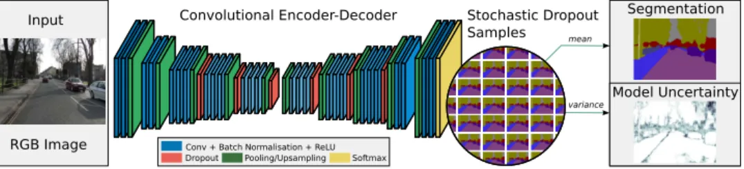
KENDALL, BADRINARAYANAN AND CIPOLLA: BAYESIAN SEGNET Convolutional Encoder-Decoder Input Segmentation Model Uncertainty Stochastic Dropout Samples

Conv + Batch Normalisation + ReLU Dropout Pooling/Upsampling Softmax

mean

variance

RGB Image

Figure 1: A schematic of the Bayesian SegNet architecture. This diagram shows the entire pipeline for the system which is trained end-to-end in one step with stochastic gradient descent. The encoders are based on the 13 convolutional layers of the VGG-16 network [27], with the decoder placing them in reverse. The probabilistic output is obtained from Monte Carlo samples of the model with dropout at test time. We take the variance of these softmax samples as the model uncertainty for each class.

probabilistic deep convolutional neural network framework for pixel-wise semantic segmen-tation. We use dropout at test time which allows us to approximate epistemic uncertainty by sampling from a Bernoulli distribution across the network’s weights. This is achieved with no additional parametrisation. In particular, we analyse which part of deep encoder decoder models benefit from Bayesian modelling.

In section 5, we demonstrate that our Bayesian approach improves performance of a number of baseline models on prominent scene understanding datasets, CamVid [3], SUN RGB-D [28] and Pascal VOC [9]. In particular, we find a larger performance improvement on smaller datasets such as CamVid where the Bayesian Neural Network is able to cope with the additional uncertainty from a smaller amount of data. Moreover, we show that this technique is broadly applicable across a number of state of the art architectures and achieves a 2-3% improvement in segmenation accuracy when applied to SegNet [2], FCN [20], Dilation Network [30] and DenseNet [15]. Finally in section5.1we demonstrate the effectiveness of model uncertainty. We explore what factors contribute to Bayesian SegNet making an uncertain prediction.

2 Related Work

Semantic pixel labelling was initially approached with TextonBoost [24], TextonForest [23] and Random Forest Based Classifiers [25]. Deep learning architectures are now the standard approach for pixel-wise segmentation, such as SegNet [2] Fully Convolutional Networks (FCN) [20] and Dilation Network [30]. FCN is trained using stochastic gradient descent with a stage-wise training scheme. SegNet was the first architecture proposed that can be trained end-to-end in one step, due to its lower parametrisation. We have also seen methods which improve on these core architectures by adding post processing tools. HyperColumn [13] and DeConvNet [22] use region proposals to bootstrap theircore segmentation engine. DeepLab [4] post-processes with conditional random fields (CRFs) and CRF-RNN [32] use recurrent neural networks. These methods improve performance by smoothing the output and ensuring label consistency. However none of these segmentation methods generate a probabilistic output with a measure of model uncertainty.

(3)

21]. They offer a probabilistic interpretation of deep learning models by inferring distribu-tions over the networks’ weights. They are often computationally very expensive, increasing the number of model parameters without increasing model capacity significantly. Perform-ing inference in Bayesian neural networks is a difficult task, and approximations to the model posterior are often used, such as variational inference [12].

On the other hand, the already significant parametrization of convolutional network ar-chitectures leaves them particularly susceptible to over-fitting without large amounts of train-ing data. A technique known asdropoutis commonly used as a regularizer in convolutional neural networks to prevent over-fitting and co-adaptation of features [29]. During training with stochastic gradient descent,dropoutrandomly removes units within a network. By do-ing this it samples from a number of thinned networks with reduced width. At test time, standard dropout approximates the effect of averaging the predictions of all these thinned networks by using the weights of the unthinned network – referred to asweight averaging.

Gal and Ghahramani [11] have interpreted dropout as approximate Bayesian inference over the network’s weights. [10] shows that dropout can be used at test time to impose a Bernoulli distribution over the convolutional net filter’s weights, without requiring any addi-tional model parameters. This is achieved by sampling the network with randomly dropped out units at test time. We can consider these as Monte Carlo samples obtained from the pos-terior distribution over models. This technique has seen success in modelling uncertainty for camera relocalisation [17]. Here we apply it to pixel-wise semantic segmentation.

In particular, MC dropout is able to capture epistemic uncertainty, which accounts for un-certainty in the model parameters – unun-certainty which captures our ignorance about which model generated our collected data [18]. Semantic segmentation models can typically only capture aleatoric uncertainty, from the entropy of the class logits, which measures noise inherent in the observations. Bayesian SegNet models epistemic uncertainty which is impor-tant for safety applications because it is required to understand examples which are different from training data [18].

3 SegNet Architecture

We briefly review the SegNet architecture [2] which we extend to produce Bayesian SegNet. SegNet is a deep convolutional encoder decoder architecture which consists of a sequence of non-linear processing layers (encoders) and a corresponding set of decoders followed by a pixel-wise classifier. Typically, each encoder consists of one or more convolutional lay-ers with batch normalisation and a ReLU non-linearity, followed by non-overlapping max-pooling and sub-sampling. The sparse encoding due to the max-pooling process is upsampled in the decoder using the max-pooling indices in the encoding sequence. This has the important advantage of retaining class boundary details in the segmented images and also reducing the total number of model parameters. The model is trained end to end using stochastic gradient descent.

We take both SegNet [2] and a smaller variant termed SegNet-Basic [2] as our base models. SegNet’s encoder is based on the 13 convolutional layers of the VGG-16 network [27] followed by 13 corresponding decoders. SegNet-Basic is a much smaller network with only four layers each for the encoder and decoder with a constant feature size of 64. We use SegNet-Basic as a smaller model for our analysis since it conceptually mimics the larger architecture.

(4)

4 Bayesian Semantic Segmentation Model

To produce a probabilistic segmentation with Bayesian SegNet, we are interested in finding the posterior distribution over the convolutional weights,W, given our observed training data

Xand labelsY.

p(W|X,Y) (1)

In general, this posterior distribution is not tractable, therefore we need to approximate the distribution of these weights [7].

We use Monte Carlo dropout samples to approximate inference in a Bayesian neural network [10]. Typically, dropout [29] was used during training to sample thinner models to regularise the network. During inference, these models were combined with weight av-eraging. In this work, we propose to use dropout during inference to obtain samples from the posterior distribution of models. Gal and Ghahramani [10] link this technique to varia-tional inference in Bayesian convoluvaria-tional neural networks, with Bernoulli distributions over the network’s weights. We leverage this method to perform probabilistic inference over our segmentation model.

This technique allows us to learn the distribution over the network’s weights,q(W), by minimising the Kullback-Leibler (KL) divergence between this approximating distribution and the full posterior;

KL(q(W)||p(W|X,Y)). (2)

where the approximating variational distributionq(Wi)for every convolutional layeri, with unitswi,j, is defined with Bernoulli distributed random variables and variational parameters,

ˆ

w, as: wi,j∼wˆi,jBernoulli(pi)for all units j. At the extreme case, if we have infinite units

for each layer our approximate model approaches a Gaussian process [10]. The dropout probabilities, pi, could be optimised. However we fix them to the standard probability of

dropping a connection as 50%, i.e.pi=0.5 [29].

In [10] it was shown that minimising the cross entropy loss objective function has the effect of minimising the Kullback-Leibler divergence term. We use this loss and train the network with stochastic gradient descent. This will encourage the model to learn a distribu-tion of weights which explains the data well while preventing over-fitting.

We train the model with dropout and sample the posterior distribution over the weights at test time using dropout to obtain the posterior distribution of softmax class probabilities. We take themean of these samples for our segmentation predictionand use thevariance to output model uncertainty for each class. We take the mean of the per-class variance measurements as an overall measure of model uncertainty. We also explored using thevariation ratioas a measure of uncertainty (i.e. the percentage of samples which agree with the class prediction) however we found this to qualitatively produce a more binary measure of model uncertainty. Fig. 1shows a schematic of the segmentation prediction and model uncertainty estimate process.

4.1 Probabilistic Variants

A fully Bayesian network should be trained with dropout after every convolutional layer. However we found in practice that this was too strong a regulariser, causing the network to learn very slowly. We therefore explored a number of variants that have different config-urations of Bayesian or deterministic encoder and decoder units. We note that an encoder unit contains one or more convolutional layers followed by a max pooling layer. A decoder

(5)

Weight Monte Carlo Training

Averaging Sampling Fit

Probabilistic Variants G C I/U G C I/U G C I/U

No Dropout 82.9 62.4 46.4 n/a n/a n/a 94.7 96.2 92.7

Dropout Encoder 80.6 68.9 53.4 81.6 69.4 54.0 90.6 92.5 86.3

Dropout Decoder 82.4 64.5 48.8 82.6 62.4 46.1 94.6 96.0 92.4

Dropout Enc-Dec 79.9 69.0 54.2 79.8 68.8 54.0 88.9 89.0 80.6

Dropout Central Enc-Dec 81.1 70.6 55.7 81.6 70.6 55.8 90.4 92.3 85.9

Dropout Center 82.9 68.9 53.1 82.7 68.9 53.2 93.3 95.4 91.2

Dropout Classifier 84.2 62.6 46.9 84.2 62.6 46.8 94.9 96.0 92.3

Table 1:Architecture Variants for SegNet-Basic on the CamVid dataset[3]. We compare the performance of weight averaging against 50 Monte Carlo samples. We quantify perfor-mance with three metrics; global accuracy (G), class average accuracy (C) and intersection over union (I/U). Results are shown as percentages (%). We observe that dropping out every encoder and decoder is too strong a regulariser and results in a lower training fit. The optimal result across all classes is when only the central encoder and decoders are dropped out.

unit contains one or more convolutional layers followed by an upsampling layer. The vari-ants are: Bayesian Encoder dropout after each encoder unit,Bayesian Decoder dropout after each decoder unit, Bayesian Encoder-Decoder dropout after each encoder and de-coder unit, Bayesian Centerdropout after the deepest encoder, before the decoder stage,

Bayesian Central Four Encoder-Decoderdropout after the central four encoder and

de-coder units andBayesian Classifierdropout after the last decoder unit, before the classifier. For analysis we use the smaller eight layer SegNet-Basic architecture [2] and test these Bayesian variants on the CamVid dataset [3]. We observe qualitatively that all six variants produce similar looking model uncertainty output. That is, they are uncertain near the border of segmentations and with visually ambiguous objects, such as cyclist and pedestrian classes. However, Table1shows a difference in quantitative segmentation performance.

We observe using dropout after all the encoder and decoder units results in a lower train-ing fit and poorer test performance as it is too strong a regulariser on the model. We find that dropping out half of the encoder or decoder units is the optimal configuration. The best configuration is dropping out the deepest half of the encoder and decoder units. We therefore benchmark our Bayesian SegNet results on the Central Enc-Dec variant. For the full 26 layer Bayesian SegNet, we add dropout to the central six encoders and decoders. This is illustrated in Fig.1.

In the lower layers of convolutional networks basic features are extracted, such as edges and corners [31]. These results show that applying Bayesian weights to these layers does not result in a better performance. We believe this is because these low level features are consistent across the distribution of models because they are better modelled with determin-istic weights. However, the higher level features that are formed in the deeper layers, such as shape and contextual relationships, are more effectively modelled with Bayesian weights.

4.2 Comparing Weight Averaging and Monte Carlo Dropout Sampling

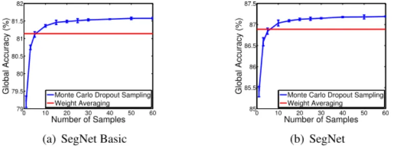
Monte Carlo dropout sampling qualitatively allows us to understand the model uncertainty of the result. However, for segmentation, we also want to understand the quantitative dif-ference between sampling with dropout and using the weight averaging technique proposed by [29]. Weight averaging proposes to remove dropout at test time and scale the weights proportionally to the dropout percentage. Fig. 2 shows that Monte Carlo sampling with

(6)

KENDALL, BADRINARAYANAN AND CIPOLLA: BAYESIAN SEGNET 0 10 20 30 40 50 60 79 79.5 80 80.5 81 81.5 82 Number of Samples Global Accuracy (%) _{Monte Carlo Dropout Sampling}

Weight Averaging

(a) SegNet Basic

0 10 20 30 40 50 60 85 85.5 86 86.5 87 87.5 Number of Samples

Global Accuracy (%) _{Monte Carlo Dropout Sampling}

Weight Averaging

(b) SegNet

Figure 2: Global segmentation accuracy against number of Monte Carlo samples for both SegNet and SegNet-Basic.Results averaged over 5 trials, with two standard deviation error bars, are shown for the CamVid dataset. This shows that Monte Carlo sampling out-performs the weight averaging technique after approximately 6 samples, and converges after approx. 40 samples.

dropout performs better than weight averaging after approximately 6 samples. We also ob-serve no additional performance improvement beyond approximately 40 samples. Therefore the weight averaging technique produces poorer segmentation results, in terms of global ac-curacy, in addition to being unable to provide a measure of model uncertainty. However, sampling comes at the expense of inference time, but when computed in parallel on a GPU this cost can be reduced for practical applications.

5 Experiments

We implement Bayesian SegNet using the Caffe library [16]. We train the whole system end-to-end using stochastic gradient descent with a base learning rate of 0.001 and weight decay parameter equal to 0.0005. Following [2] we train SegNet with median frequency class balancing using the formula proposed by Eigen and Fergus [8]. We use batch normalisation after every convolutional layer [14].

We quantify the performance of Bayesian SegNet on three different benchmarks using our Caffe implementation. Through this process we demonstrate the efficacy of Bayesian SegNet for a wide variety of scene segmentation tasks which have practical applications. CamVid [3] is a road scene understanding dataset which has applications for autonomous driving. SUN RGB-D [28] is a very challenging and large dataset of indoor scenes which is important for domestic robotics. Finally, Pascal VOC 2012 [9] is a RGB dataset for object segmentation.

CamVidis a road scene understanding dataset with 367 training images and 233 testing

images of day and dusk scenes [3] with 11 classes. We resize images to 360x480 pixels for training and testing of our system. We show our Bayesian method outperforms other models in Table2with qualitative results in Fig.5.

SUN RGB-D[28] is a challenging and large dataset of indoor scenes with 5285 training

and 5050 testing images. The images are captured by different sensors and are labelled with 37 indoor semantic classes. Table2 and Fig. 4compare to other models, including those which use depth input. Our method outperforms all of these other techniques. We also note that an earlier benchmark dataset, NYUv2 [26], is included as part of this dataset.

(7)

Figure 3:Bayesian SegNet results on CamVid dataset [3].From top: input image, ground truth, Bayesian SegNet’s segmentation prediction, and overall model uncertainty averaged across all classes (with darker colours indicating more uncertain predictions).

Figure 4: Bayesian SegNet results on the SUN RGB-D dataset [28].Bayesian SegNet uses only RGB input and is able to accurately segment 37 classes in this challenging dataset.

(8)

KENDALL, BADRINARAYANAN AND CIPOLLA: BAYESIAN SEGNET CamVid G C I/U SegNet-Basic [2] 82.8 62.3 46.3 SegNet [2] 88.6 65.9 50.2 FCN 8 [20] 83.1 64.2 52.0 DeconvNet [22] 85.9 62.1 48.9 DeepLab-LargeFOV-DenseCRF [4] 89.7 60.7 54.7 DenseNet [15] 91.5 - 66.9

Bayesian SegNet Models in this work:

Bayesian SegNet-Basic 81.6 70.5 55.8

Bayesian SegNet 86.9 76.3 63.1

Bayesian DenseNet 91.9 - 67.2

SUN RGB-D G C I/U

RGB

Liuet al.[19] n/a 9.3 n/a

FCN 8 [20] 68.2 38.4 27.4

DeconvNet [22] 66.1 32.3 22.6 DeepLab-LargeFOV-CRF [4] 67.0 33.0 24.1

SegNet [2] 70.3 35.6 22.1

Bayesian SegNet(this work) 71.2 45.9 30.7 Table 2:Quantitative resultsfor CamVid [3] (left) and SUN RGB-D [28] (right).

Pascal VOC12 segmentation challenge [9] consists of segmenting 20 salient object

classes from widely varying backgrounds. We train on the 12031 training images and 1456 testing images. Table3shows our results compared to other methods, with qualitative results in Fig.5.

To demonstrate the general applicability of this method, we also apply it to other deep learning architectures trained with dropout; FCN [20] and Dilation Network [30]. We select these state-of-the-art methods as they are already trained by their respective authors using dropout. We take their trained, open source models off the shelf, and evaluate them using 50 Monte Carlo dropout samples. Table3shows the mean IoU result of these methods evaluated as Bayesian Neural Networks, as computed by the online evaluation server. This shows the general applicability of our method. By leveraging this underlying Bayesian framework our method obtains 2-3% improvement across this range of architectures.

Parameters Pascal VOC Test IoU

Method (Millions) Non-Bayesian Bayesian

Dilation Network [30] 140.8 71.3 73.1

FCN-8 [20] 134.5 62.2 65.4

SegNet [2] 29.45 59.1 60.5

Table 3: Pascal VOC12 [9] test resultsevaluated from the online evaluation server. We compare to competing deep learning architectures. Bayesian SegNet is considerably smaller but achieves a competitive accuracy to other methods. We also evaluate FCN [20] and Di-lation Network (front end) [30] with Monte Carlo dropout sampling. We observe a 2-3% improvement in segmentation performance across all three deep learning models when us-ing the Bayesian approach.

5.1 Understanding Model Uncertainty

Qualitative observations. Fig. 5shows segmentations and model uncertainty results from

Bayesian SegNet on CamVid Road Scenes [3]. Fig. 4 shows SUN RGB-D Indoor Scene

Understanding [28] results and Fig. 5has Pascal VOC [9] results. These figures show the qualitative performance of Bayesian SegNet. We observe that segmentation predictions are smooth, with a sharp segmentation around object boundaries. Also, when the model predicts an incorrect label, the model uncertainty is generally very high. More generally, we observe that a high model uncertainty is predominantly caused by three situations.

Firstly, at class boundaries the model often displays a high level of uncertainty. This reflects the ambiguity surrounding the definition of defining where these labels transition. The Pascal results clearly illustrated this in Fig.5.

(9)

(a) Performance vs. mean model uncertainty (b) Class frequency vs. mean model uncer-tainty

Figure 6: Bayesian SegNet performance and frequency compared to mean model un-certaintyfor each class in CamVid road scene understanding dataset. These figures show a strong inverse relationships. We observe in (a) that the model is more confident with more accurate classes. (b) shows classes that Bayesian SegNet is more confident at are more preva-lent in the dataset. Conversely, for the more rare classes such as Sign Symbol and Bicyclist, Bayesian SegNet has a much higher model uncertainty.

Secondly, objects which are visually difficult to identify often appear uncertain to the model. This is often the case when objects are occluded or at a distance from the camera.

The third situation causing model uncertainty is when the object appears visually am-biguous to the model. As an example, cyclists in the CamVid results (Fig. 5) are visually similar to pedestrians, and the model often displays uncertainty around them. We observe similar results with visually similar classes in SUN (Fig.4) such as chair and sofa, or bench and table. In Pascal this is often observed between cat and dog, or train and bus classes.

Quantitative observations. To understand what causes the model to be uncertain, we

have plotted the relationship between uncertainty and accuracy in Fig.6(a)and between un-certainty and the frequency of each class in the dataset in Fig.6(b). Uncertainty is calculated as the mean uncertainty value for each pixel of that class in a test dataset. We observe an inverse relationship between uncertainty and class accuracy or class frequency. This shows that the model is more confident about classes which are easier or occur more often, and less certain about rare and challenging classes.

6 Conclusions

We have presented Bayesian SegNet, the first probabilistic framework for semantic segmen-tation using deep learning, which outputs a measure of model uncertainty for each class. We show that the model is uncertain at object boundaries and with difficult and visually ambiguous objects.

We quantitatively show Bayesian SegNet produces a reliable measure of model uncer-tainty, improving segmentation performance by 2-3% across a number of state of the art architectures such as SegNet, FCN and Dilation Network, while requiring no additional pa-rameters. We demonstrate how to apply our knowledge of uncertainty to active learning which significantly reduces the requirement for expensive labelled data. For future work we intend to explore how video data can improve our model’s performance.

(10)

References

[1] Vijay Badrinarayanan, Fabio Galasso, and Roberto Cipolla. Label propagation in video sequences. InComputer Vision and Pattern Recognition (CVPR), 2010 IEEE Confer-ence on, pages 3265–3272. IEEE, 2010.

[2] Vijay Badrinarayanan, Alex Kendall, and Roberto Cipolla. Segnet: A deep

con-volutional encoder-decoder architecture for image segmentation. arXiv preprint arXiv:1511.00561, 2015.

[3] Gabriel J Brostow, Julien Fauqueur, and Roberto Cipolla. Semantic object classes in video: A high-definition ground truth database. Pattern Recognition Letters, 30(2): 88–97, 2009.

[4] Liang-Chieh Chen, George Papandreou, Iasonas Kokkinos, Kevin Murphy, and Alan L Yuille. Semantic image segmentation with deep convolutional nets and fully connected crfs.arXiv preprint arXiv:1412.7062, 2014.

[5] David A Cohn, Zoubin Ghahramani, and Michael I Jordan. Active learning with statis-tical models. Journal of artificial intelligence research, 1996.

[6] Camille Couprie, Clément Farabet, Laurent Najman, and Yann LeCun. Indoor semantic segmentation using depth information.arXiv preprint arXiv:1301.3572, 2013. [7] John Denker and Yann Lecun. Transforming neural-net output levels to probability

distributions. InAdvances in Neural Information Processing Systems 3. Citeseer, 1991.

[8] David Eigen and Rob Fergus. Predicting depth, surface normals and

seman-tic labels with a common multi-scale convolutional architecture. arXiv preprint arXiv:1411.4734, 2014.

[9] Mark Everingham, Luc Van Gool, Christopher KI Williams, John Winn, and Andrew Zisserman. The pascal visual object classes (voc) challenge. International journal of computer vision, 88(2):303–338, 2010.

[10] Yarin Gal and Zoubin Ghahramani. Bayesian convolutional neural networks with

bernoulli approximate variational inference.arXiv:1506.02158, 2015.

[11] Yarin Gal and Zoubin Ghahramani. Dropout as a Bayesian approximation: Represent-ing model uncertainty in deep learnRepresent-ing.arXiv:1506.02142, 2015.

[12] Alex Graves. Practical variational inference for neural networks. InAdvances in Neural Information Processing Systems, pages 2348–2356, 2011.

[13] Bharath Hariharan, Pablo Arbeláez, Ross Girshick, and Jitendra Malik. Hypercolumns for object segmentation and fine-grained localization.arXiv preprint arXiv:1411.5752, 2014.

[14] Sergey Ioffe and Christian Szegedy. Batch normalization: Accelerating deep network training by reducing internal covariate shift.arXiv preprint arXiv:1502.03167, 2015. [15] Simon Jégou, Michal Drozdzal, David Vazquez, Adriana Romero, and Yoshua Bengio.

The one hundred layers tiramisu: Fully convolutional densenets for semantic segmen-tation.arXiv preprint arXiv:1611.09326, 2016.

(11)

[16] Yangqing Jia, Evan Shelhamer, Jeff Donahue, Sergey Karayev, Jonathan Long, Ross Girshick, Sergio Guadarrama, and Trevor Darrell. Caffe: Convolutional architecture for fast feature embedding.arXiv preprint arXiv:1408.5093, 2014.

[17] Alex Kendall and Roberto Cipolla. Modelling uncertainty in deep learning for camera relocalization.arXiv preprint arXiv:1509.05909, 2015.

[18] Alex Kendall and Yarin Gal. What uncertainties do we need in bayesian deep learning for computer vision?arXiv preprint arXiv:1703.04977, 2017.

[19] Ce Liu, Jenny Yuen, Antonio Torralba, Josef Sivic, and William T Freeman. Sift flow: Dense correspondence across different scenes. InComputer Vision–ECCV 2008, pages 28–42. Springer, 2008.

[20] Jonathan Long, Evan Shelhamer, and Trevor Darrell. Fully convolutional networks for semantic segmentation.arXiv preprint arXiv:1411.4038, 2014.

[21] David JC MacKay. A practical bayesian framework for backpropagation networks. Neural computation, 4(3):448–472, 1992.

[22] Hyeonwoo Noh, Seunghoon Hong, and Bohyung Han. Learning deconvolution net-work for semantic segmentation.arXiv preprint arXiv:1505.04366, 2015.

[23] Jamie Shotton, Matthew Johnson, and Roberto Cipolla. Semantic texton forests for image categorization and segmentation. InComputer vision and pattern recognition, 2008. CVPR 2008. IEEE Conference on, pages 1–8. IEEE, 2008.

[24] Jamie Shotton, John Winn, Carsten Rother, and Antonio Criminisi. Textonboost for image understanding: Multi-class object recognition and segmentation by jointly mod-eling texture, layout, and context. International Journal of Computer Vision, 81(1): 2–23, 2009.

[25] Jamie Shotton, Toby Sharp, Alex Kipman, Andrew Fitzgibbon, Mark Finocchio, An-drew Blake, Mat Cook, and Richard Moore. Real-time human pose recognition in parts from single depth images.Communications of the ACM, 56(1):116–124, 2013. [26] Nathan Silberman, Derek Hoiem, Pushmeet Kohli, and Rob Fergus. Indoor

segmenta-tion and support inference from rgbd images. InComputer Vision–ECCV 2012, pages 746–760. Springer, 2012.

[27] Karen Simonyan and Andrew Zisserman. Very deep convolutional networks for large-scale image recognition.arXiv preprint arXiv:1409.1556, 2014.

[28] Shuran Song, Samuel P Lichtenberg, and Jianxiong Xiao. Sun rgb-d: A rgb-d scene understanding benchmark suite. InProceedings of the IEEE Conference on Computer Vision and Pattern Recognition, pages 567–576, 2015.

[29] Nitish Srivastava, Geoffrey Hinton, Alex Krizhevsky, Ilya Sutskever, and Ruslan Salakhutdinov. Dropout: A simple way to prevent neural networks from overfitting. The Journal of Machine Learning Research, 15(1):1929–1958, 2014.

[30] Fisher Yu and Vladlen Koltun. Multi-scale context aggregation by dilated convolutions. InICLR, 2016.

(12)

[31] Matthew D Zeiler and Rob Fergus. Visualizing and understanding convolutional net-works. InComputer Vision–ECCV 2014, pages 818–833. Springer, 2014.

[32] Shuai Zheng, Sadeep Jayasumana, Bernardino Romera-Paredes, Vibhav Vineet, Zhizhong Su, Dalong Du, Chang Huang, and Philip Torr. Conditional random fields as recurrent neural networks.arXiv preprint arXiv:1502.03240, 2015.