Scale up Vs. Scale out in Cloud Storage and
Graph Processing Systems
Wenting Wang, Le Xu, Indranil Gupta
Department of Computer Science, University of Illinois, Urbana Champaign
{wwang84, lexu1, indy}@illinois.edu
Abstract—Deployers of cloud storage and iterative processing systems typically have to deal with either dollar budget constraints or throughput requirements. This paper examines the question of whether such cloud storage and iterative processing systems are more cost-efficient when scheduled on a COTS (scale out) cluster or a single beefy (scale up) machine. We experimentally evaluate two systems: 1) a distributed key-value store (Cassandra), and 2) a distributed graph processing system (GraphLab). Our studies reveal scenarios where each option is preferable over the other. We provide recommendations for deployers of such systems to decide between scale up vs. scale out, as a function of their dollar or throughput constraints. Our results indicate that there is a need for adaptive scheduling in heterogeneous clusters containing scale up and scale out nodes.
I. INTRODUCTION
Today’s public clouds offer a bewildering array of choices for compute instances. The compute instances offered by public clouds such as AWS, Microsoft Azure, Google Compute En-gine, as well as by private clouds, cover a large range in terms of their capacity (CPU, RAM, and storage) and associated costs. For instance, AWS offers virtualized instances ranging from the wimpy and cheap—m3.medium offers 1 CPU, 3.75 GB of RAM, and 1 x 4 GB SSD of storage for $0.07 per hour—to the beefy and expensive—i2.8xlarge with 32 CPUs, 244 GB of RAM and 8 x 800 GB of storage for $6.82 per hour.
This makes it challenging for deployers to reason about which instances are the best for their individual application. In fact, deployers are often faced with dollar budget caps or minimum throughput requirements for their applications. They have to choose between wimpy and beefy nodes by relying on coarse-grained suggestions [1]. Moreover, the type of application highly influences the choice of machines. Storage systems tend to choose memory- and storage-optimized machines while computation-intensive systems may choose machines with fast CPUs. Further, we are far from knowing how to schedule such applications dynamically on a highly heterogeneous cluster containing both wimpy and beefy machines.
In this paper, we choose two typical applications for cloud storage and computation systems: 1) Apache Cassandra [17], the most popular open-source distributed key-value store, and 2) GraphLab [18], a popular open-source distributed graph processing system. We quantify their performance on two types
of clusters: a COTS or scale out cluster infrastructure with
several relatively wimpy machines, and ascale upoption with
This work was supported in part by the following grants: NSF CNS1319527, NSF CCF 0964471, NSF CNS 1409416, and AFOSR/AFRL FA 8750-11-2-0084.
one beefy machine. The primary metric for this comparison is a normalized metric called cost-efficiency, i.e., the ratio of performance to dollar cost. In order to retain our focus on performance, we defer orthogonal issues such as fault-tolerance. For our results to be generalizable across different infras-tructures, we first perform a linear regression analysis of the costs offered by the three biggest providers of public clouds: AWS [2], Microsoft Azure [5], and Google Compute Engine (GCE) [4]. This allows us to derive for the operational cost of a machine with arbitrary specifications. We then apply these cost functions while running our experiments on two clusters: Emulab [3] as the scale out cluster, and a local cluster at Illinois named Mustang for scale up.
Unlike previous studies on Hadoop which found scale up generally preferable for small jobs [7], our experiments find that under some scenarios scale out is the more preferable option in Cassandra and GraphLab. We provide a series of recommendations for deployers of cloud systems who may be faced with either a dollar budget limit or a minimum throughput requirement, allowing them to choose scale up or scale out.
Finally, we explore implications for applications that would like to use a heterogeneous mix of machines, i.e., a few scale up machines mixed with a few scale out machines. We believe there is significant room for innovation in adaptive scheduling techniques in heterogeneous cluster.
II. EXPERIMENTSETUP
We collected the hourly costs of instances from three public cloud providers on May 11th, 2014: AWS, Microsoft Azure, and Google Compute Engine. We performed linear least squares regression for each provider. Cost of cloud providers grows linearly with resource quantity, and this motivates our choice of the linear model. This enables us to derive cost models for instances as a linear combination of three components: i) number of CPUs times the GHz, ii) RAM (GB), and iii) storage (with separate cost functions for hard disk vs. SSD).
Table 1 shows the per-unit costs for each of the above three components. Since Azure and GCE do not provide SSD pricing, we use industry rules of thumb to derive SSD cost [14].
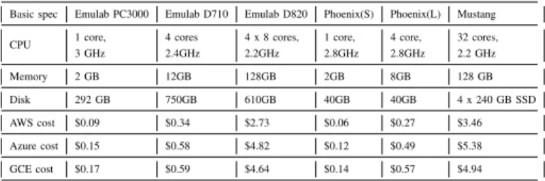
We performed our experiments on three environments: i) the Emulab PC3000 and D170 machines over a 100 Mbps Ethernet for scale out; ii) a local machine called Mustang for scale up, and iii) a heterogeneous local cluster called Phoenix with VMs for Cassandra, and Emulab for GraphLab. The specifications of these machines are listed in Table II, along with their component-wise costs for three providers, based on Table I.
TABLE I: Component unit price for 3 providers
$/GHz $/GB $/TB (HDD, SSD) AWS (HDD, SSD) (0.0141, 0.0085) (0.0106, 0.0208) 0.10,0.20 Azure 0.0302 0.0181 (0.10,0.97) GCE 0.0442 0.0101 (0.06,0.56)
TABLE II: Clusters/single node used in our experiments, and their costs for the three providers from Table 1.
Basic spec Emulab PC3000 Emulab D710 Emulab D820 Phoenix(S) Phoenix(L) Mustang
CPU 1 core, 3 GHz 4 cores 2.4GHz 4 x 8 cores, 2.2GHz 1 core, 2.8GHz 4 core, 2.8GHz 32 cores, 2.2 GHz Memory 2 GB 12GB 128GB 2GB 8GB 128 GB Disk 292 GB 750GB 610GB 40GB 40GB 4 x 240 GB SSD AWS cost $0.09 $0.34 $2.73 $0.06 $0.27 $3.46 Azure cost $0.15 $0.58 $4.82 $0.12 $0.49 $5.38 GCE cost $0.17 $0.59 $4.64 $0.14 $0.57 $4.94
III. KEY-VALUESTOREEXPERIMENTS
To evaluate the performance of a key-value store under both scale up and scale out environment key-value store, we inject queries from multiple YCSB [10] client threads to both a scale out cluster and a running Cassandra. The workloads consist of 50% read and 50% write operations and follow a Zipf popularity distribution. The results are collected from a workload of 1 million operations on a 1 GB database. For scale up setting we assume the server is capable of storing the dataset used by any given workflow. The requests are initiated by client threads running on another disjoint but similar machine using the same network setting.
In order to provide a deeper perspective of how hardware setting and workload impact the performance of a key-value store, we vary the number of client threads (up to 96 threads) and the number of servers in the scale out cluster (up to 16 servers). The cost of a given workload is calculated as the total price (in dollars) spent over a million operations. For a real cluster, the throughput would be calculated from a long-term average. Cost-efficiency is computed as the throughput of the workload divided by the hourly cost of the cluster.
A. Scale out VS. Scale up
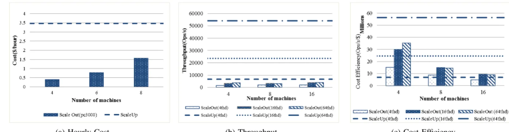
In this section we explore the performance of a key-value store under both scale up and scale out settings. Fig. 1a plots the one-hour cost of renting a scale up machine and scale out cluster of 3 different sizes based on AWS pricing discussed in Section 2. As the size of scale out cluster doubles, the cost doubles as well. Fig. 1b plots the throughput of Cassandra under workloads with different intensities (light workload using 4 client threads, medium workload using 16 client threads and intense workload using 64 threads), with different number of machines in the cluster. Fig. 1b indicates that in both scale out and scale up settings, increasing the number of client threads improves storage throughput, provided that CPU utilization does not exceed 100%. For scale out settings, the throughput also scales linearly with the number of machines in the cluster. The scale up machine produces a significantly higher throughput than scale out under all workload intensities, irrespective of cluster size.
Fig. 1c plots the cost-efficiency of two settings. From Fig. 1c we can conclude that scaling out with a small number of
machines has a higher cost-efficiency under light workload. However, the scale out cluster become less competitive in cost-efficiency when the cluster size grows. This is because the growth of the throughput is exceeded by the growth of cluster cost. Under intense workload, the scale up cluster always shows a higher cost efficiency.
Fig. 2a shows while the number of clients is less than 32, a small size cluster (4 nodes) achieves higher cost efficiency than the scale up machine. However, when the workload is intensive, scaling up significantly outperforms scaling out. To find out the impact of the number of queries on Cassandra’s cost efficiency, we present experimental results demonstrated in Fig. 2b. The results show no significant difference as the number of queries is varied.
Based on this data, we present our recommendations in Table III for applications that are either constrained by their total budget, or has minimum throughput requirements. For each of scenarios, we consider which choices of scale up vs. scale out configurations first meets the constraint. Then among these, we select option which maximizes the cost-efficiency, i.e., the throughput per dollar. Scale up is always preferable under intense workload for both constraints. This is because of the low server cost resulting from short run time of workload and the 10 times higher throughput offered by the scale up server. A scale out cluster with a small number of machines offers higher cost efficiency under light workload (Fig. 1c). Scale-up server has lower cost efficiency under such workload. This is due to the fact that its high CPU power is not being fully utilized but the hardware configuration generates a higher cost. Thus we conclude that when low throughput requirement is needed, scale out is preferable under budget constraint. Otherwise, scale up is preferred due to its high cost efficiency.
TABLE III: Cassandra: Scale up vs Scale out Recommendations for Constrained Users
Budget-constrained Min throughput requirement
Small Jobs Scale out with small number of nodes
If(low throughput requirement) Scale out with small number of nodes Else
Scale up
Large jobs Scale up Scale up
B. Heterogeneous cluster
Cassandra assigns multiple virtual nodes, called (vnodes) to distribute the keyspace more evenly across servers. In this section we discuss the performance of Cassandra under het-erogeneous environment with the cluster composed of wimpy and beefy machines. Specifically, we examine the impact of Cassandra’s vnode settings on cluster performance. We further extend our experiment to discover the relationship between optimized vnode settings and the price of machines of different configurations. Finally, we perform an experiment to explore the strategies for users constructing heterogeneous cluster with a fixed budget.
The test machines we used for heterogeneous cluster are Phoenix virtual machines with two configurations: Phoenix(L) and Phoenix(S). Phoenix(L) has 4 times the CPU power and memory of Phoenix(S). Based on the linear pricing model discussed in Section 2 (see Table II), the cost of Phoenix(L)
(a) Hourly Cost (b) Throughput (c) Cost Efficiency
Fig. 1: Cost, throughput and cost-efficiency of cassandra on scale up and scale out varied by number of client threads.
(a)Cost-Efficiency vs. Number of Client Threads Varied By Cluster Size (b)Cost-Efficiency vs. Number of Threads Varied by Number of Queries
Fig. 2: Cassandra scale up vs. scale out cluster cost efficiency varied by number of client threads and storage size.
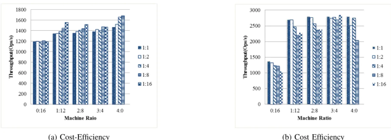
(a)Cost-Efficiency vs. Machine Ratio (Phoenix(L) : Phoneix(S) (b)Cost-Efficiency
Fig. 3: Cost-efficiency varied by cluster settings and by vnode rate (1 Phoenix(L)+12 Phoenix(S)). compared to Phoenix(S) is 4:1. For experiments of
hetero-geneous cluster, the three major parameters we vary are the number of client threads, the vnode ratio (computed as the ratio of the number of vnodes in one wimpy machine to the number of vnodes in one beefy machine), and the machine ratio (computed as the ratio of the number of beefy machines to the number of wimpy machine in the cluster).
Fig. 3a shows the cost efficiency of heterogeneous cluster with 4, 16 and 64 client threads injecting requests respectively. The vnode ratio of the wimpy machine to the beefy machine is set to 1:4 and the total cluster price is fixed. We observe that under any workload, cost efficiency of the cluster grows significantly when the first beefy node is added. Thereafter, adding further scale of nodes yields lower marginal benefit. This is because a beefy machine stores more data than a wimpy machine based on the vnode setting and the former can serve
queries locally. From Fig. 3a we also discovered that for a given cost, a homogeneous cluster of beefier machines (machine ratio 0:16) produces a better throughput than a cluster with wimpier machines (machine ratio 4:0).
Fig. 3b shows the cost-efficiency of a heterogeneous cluster varied by vnode ratio and workload. The cluster contains 1 beefy machine and 12 wimpy machines. We can observe from the plot that when the workload is relatively small, increasing the number of vnodes in beefy machines (which indicates a larger portion of Cassandra’s key space) increases cost- effi-ciency of the entire cluster. Such improvement is not exhibited under heavier workload using 16 threads and 64 threads. This is because as the vnode ratio grows, the beefy machine(s) in the cluster are likely to reach a CPU utilization of 100% quickly under intense load and thus become the bottleneck for the entire system. Fig. 4a and 4b further illustrate this fact by showing
(a) Cost-Efficiency (b) Cost Efficiency
Fig. 4: Cost-efficiency varied by cluster settings and by vnode rate (Phoenix 1L+Phoenix 12S); a positive correlation between the vnode ratio and the system
throughput under light workload and a negative correlation under intense workload, regardless of the ratio of the number of beefy machines to wimpy machines in the system.
Based on these experiments we found no clear relationship between the optimized vnode ratio and the price of a machine. Rather, we can conclude that when users are choosing the vnode ratio of the heterogeneous cluster, the ratio should be as high as possible as long as the beefy node does not cause CPU utilization to cross 100%. For a cluster with fixed price, the first beefy machine is essential to improve the cost efficiency of the entire cluster, but adding further machines has decreasing marginal benefit.
IV. GRAPHPROCESSINGEXPERIMENTS
We ran the GraphLab [18] distributed graph processing engine on the scale out cluster and on the scale up machine separately. We consider five types of graph benchmarks: i) Al-ternating least squares (ALS) [23], a powerful user recommen-dation algorithm, ii) Directed Triangle Count, iii) Connected Component Count, iv) Single Source Shortest Path (SSSP), and v) Page Rank with 10 iterations. The benchmarking job was run on four graphs (shown in Table IV): i) a small Netflex dataset, ii) Pokec [22] social network from Slovakia, iii) a graph from the LiveJournal [8] blog community of 10 million members, and iv) a Twitter graph [15].
TABLE IV: Real-world Graphs Considered in our Experiments
Graph Input |V| |E| Netflix 42M 0.09M 3.8M Poket 404M 1.6M 30M LiveJournal 1030M 4.8M 68M Twitter 6GB 41.6M 1.5G
A. Scale out Vs. Scale up
In this section, we compare two scale out clusters (PC3000 cluster and D710 cluster on Emulab) vs. a single scale up machine (Mustang with 32 cores and 128GB RAM). Due to space constraints, and because the trends and conclusions are similar for many combinations, we only present PageRank results on two graphs using the AWS cost function.
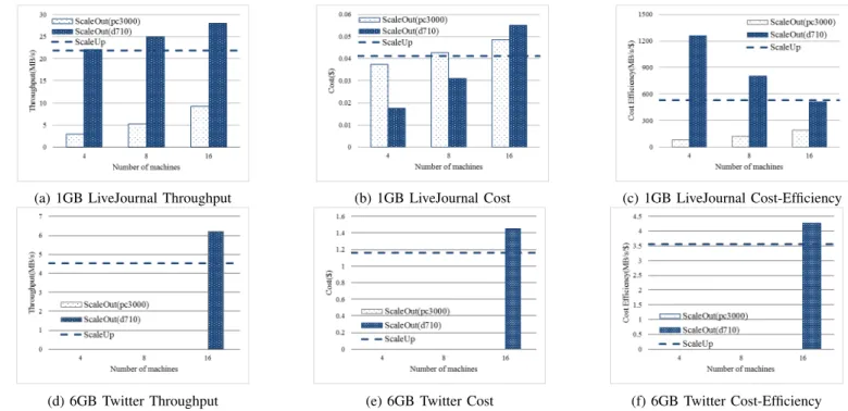
Fig. 5 shows the raw throughput, total cost and cost-efficiency of running PageRank on 1 GB LiveJournal and 6 GB Twitter graph respectively.
For a small job (Fig. 5a - 5c), the throughput scales nonlin-early on D710 but linnonlin-early on PC3000 scale out cluster as the cluster size grows. D710 cluster’s throughput growth is limited by some certain stages of graph processing where only one core per machine is used (e.g., only one core is used for parsing input). However, the throughput of PC3000 cluster, which only has one core per machines, scale linearly. Moreover, for D710 cluster, its throughput growth is limited by The throughput The 4-D710 cluster has similar throughput as the scale up machine since they have the same number of cores (scale up machine has 16 cores and 4-D710 cluster has 4 x 4 cores). The scale out cluster which parses data in parallel is faster than scale up. PC3000 scale out cluster performs worse than the single scale up machine. One reason is that PC3000 (scale out) has only one core and it is not the optimal configuration for GraphLab. Another reason is that the memory of PC3000 (scale out) cluster is not large enough to hold the entire graph [13]. For a large job (Fig. 5d - 5f), GraphLab could not load the graph at all kinds of PC-3000 clusters and 4 or 8-D710 cluster. PageRank on the Twitter graph only works well on a 16-D710 cluster. Distributed graph processing on multiple machines requires more memory than on a single machine, since some vertices of the graph need to be replicated among machines [18]. So a scale out cluster with a small number of machines may suffer out-of-memory error and not be able to load a large graph.
For cost in Fig. 5b, it is interesting that the small D710 cluster is the cheapest when job size is small. The scale up machine suffers from the high price per unit time, which is partly due to the high-cost SSD. The PC3000 cluster that has the lowest unit price, however, has a longer job completion time which generates a higher total cost. When job size is large (Fig. 5e), since no small scale out cluster could perform the computation, the scale up machine becomes the cheapest.
In terms of cost-efficiency, when job size is small (Fig. 5c), the small D710 scale out cluster provides better cost-efficiency compared to the scale up machine. One reason is that the small job running on the scale up machine does not make the best use of powerful and expensive CPUs. Another reason is the expensive SSD in the scale up machine helps little in computation-intensive jobs. When job size is large (Fig. 5f), the large scale out cluster shows better cost-efficiency. Although the 4-D710 cluster is more expensive than the scale up machine, it achieves a better performance on the large graph by parallelizing
(a) 1GB LiveJournal Throughput (b) 1GB LiveJournal Cost (c) 1GB LiveJournal Cost-Efficiency
(d) 6GB Twitter Throughput (e) 6GB Twitter Cost (f) 6GB Twitter Cost-Efficiency
Fig. 5:Cost, throughput and cost-efficiency on scale up and scale out with PageRank running on small 1GB LiveJournal and large 6GB Twitter Graph. Cost = $ per hour per node x the number of nodes x the completion time of the job. Each plotted data point is the average of 3 trials.
TABLE V: GraphLab: Scale up vs Scale out Recommendations for Constrained Users
Budget-constrained Min throughput requirement
Small Jobs Scale out with
small number of nodes
Scale out with small number of nodes
Large jobs Scale up Scale out
with large number of nodes
the computation.
Based on this data, we present our recommendations for throughput- and budget-constrained applications in Table V. These conclusions are different from the recommendation for Cassandra (Table III). In particular, when the application has a minimum throughput need, we always recommend scale out because its throughput is higher than scale up (Figs. 5b and 5e). For small graphs, a scale out cluster with a small number of machines is preferable as it has comparable cost efficiency (Fig. 5c). For large graphs, a powerful scale out cluster with a large number of machines is better as it provides sufficient memory. On the other hand, when the constraint is budget, scale up is preferable when processing large graphs. If graph is small, our recommendation is generally to prefer small scale out cluster (which have multi-core configuration) because this option incurs lower cost in Fig. 5c.
B. Heterogeneous cluster
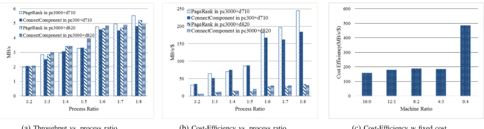
In this section, we study the performance and cost-efficiency of GraphLab running in a heterogeneous cluster with one beefy machine (D710 or D820) and a wimpy machine (PC3000) in Figs. 6a and 6b. We run only one GraphLab process on a wimpy machine and vary the number of processes running on a more powerful machine. The performance of the whole cluster is improved in Fig. 6a as we run more computation processes in the powerful machine. This leads to an improvement of cost-efficiency (Fig. 6b) because the beefy node in the cluster is better utilized.
Fig. 6c shows the cost efficiency of PageRank running on a cluster when the total cost is fixed. As shown in Table II, a D710 is almost four times as expensive as PC3000. With a fixed budget (e.g., 16 x $0.09 = $1.44), one can rent a 16-PC3000 cluster, or a 4-D710 cluster, or a heterogeneous cluster with a mix of PC3000 and D710. We run one GraphLab process on PC3000 and four processes on D710. The experimental result shows that a 4-D710 cluster provides the best cost efficiency. The reason is similar to Section IV-A. That is, PC3000’s single core configuration is not optimal for GraphLab. Consequently, in a heterogeneous cluster, PC3000s become stragglers which slow down the whole computation process.
Based on these experiments, we concluded that running more computation processes on a beefy machine in the heterogeneous cluster improves the overall performance and cost-efficiency. With fixed budget, the proportion of beefy machines in the cluster should be as high as possible.
V. RELATEDWORK
Analytics: MapReduce is designed for parallel data process-ing tasks. The typical deployment leverages a cheap commodity cluster in a scale out manner. However, it also suffers from network bottleneck due to shuffling intermediate data. There are also some in-memory multi-core optimized MapReduce libraries, such as Phoenix [21], Metis [20], and TiledMapReduce [9], which show that a scale up solution can be implemented in a shared-memory multi-threaded manner. This tradeoff between scale up and scale out was explicitly studied by Appuswamy et al. [7] work. They showed that Hadoop jobs are often better served by a scale-up server rather than a scale out cluster.
Storage: DeWitt and Gray demonstrated in [11] that with disk and processor speed developing rapidly, parallel systems may become a popular solution for future distributed storage perform better and achieve better fault tolerance. Anderson et al. [6] pointed out that the scale up machine can be inefficient in terms of power consumption.
(a)Throughput vs. process ratio (b)Cost-Efficiency vs. process ratio (c)Cost-Efficiency w fixed cost
Fig. 6: Throughput and cost-efficiency of PageRank and ConnectedComponentCount on two heterogeneous clusters (PC3000+D710 and
PC3000+D820); and Cost-efficiency of PageRank when running on different clusters with fixed cost.
Graph processing: Distributed graph processing systems such as GraphLab [18], PowerGraph [12], Pregel [19], LFGraph [13], perform analysis on huge graphs in parallel to improve performance. However, they still suffer from network com-munication overhead and redundant storage of vertices/edges. GraphChi [16] advocates processing graph on a single server. However, GraphChi uses disk, which makes it slower than in-memory operations.
VI. CONCLUSION
Previous studies on scale up vs. scale out for Hadoop [7] did not look at budget or throughput constraints. In comparison, we conclude that for key-value stores and graph processing systems, only two options are feasible: scale up, or small to medium scale out clusters. The choice between scale up vs. scale out is sensitive to the type of application (stream vs. graph processing) and parameters such as workload intensity, job size, dollar budget, and throughput requirements. While we have considered throughput and completion time as the primary metrics, similar studies can be performed on other metrics such as latency and resource utilization. These might yield interesting (and possibly different) conclusions.
Today, most application deployers have the opportunity to run heterogeneous clusters consisting of both wimpy (scale out) nodes alongside a small number of beefy (scale up) nodes. Our study thus opens up an opportunity to innovate in adaptive algorithms and techniques which obey the deployer constraints such as budget or throughput.
REFERENCES
[1] AWS User Guide: Choosing Reserved Instances Based on your Usage Plans. http://docs.aws.amazon.com/AWSEC2/latest/UserGuide/reserved-instances-offerings.html.
[2] EC2. http://aws.amazon.com/ec2/. [3] Emulab. http://www.emulab.net/.
[4] Google Computer Engine Pricing. https://developers.google.com/compute/ pricing.
[5] Microsoft Azure Linux Pricing. http://www.windowsazure.com/en-us/ pricing/details/virtual-machines/#linux.
[6] David G Andersen, Jason Franklin, Michael Kaminsky, Amar Phan-ishayee, Lawrence Tan, and Vijay Vasudevan. Fawn: A fast array of wimpy nodes. InProceedings of the ACM SIGOPS 22nd symposium on Operating systems principles, pages 1–14. ACM, 2009.
[7] Raja Appuswamy, Christos Gkantsidis, Dushyanth Narayanan, Orion Hodson, and Antony Rowstron. Scale-up vs scale-out for hadoop: Time to rethink? In Proceedings of the 4th annual Symposium on Cloud Computing, page 20. ACM, 2013.
[8] Lars Backstrom, Dan Huttenlocher, Jon Kleinberg, and Xiangyang Lan. Group formation in large social networks: membership, growth, and evolution. In Proceedings of the 12th ACM SIGKDD international conference on Knowledge discovery and data mining, pages 44–54. ACM, 2006.
[9] Rong Chen, Haibo Chen, and Binyu Zang. Tiled-mapreduce: optimizing resource usages of data-parallel applications on multicore with tiling. In Proceedings of the 19th international conference on Parallel architectures and compilation techniques, pages 523–534. ACM, 2010.
[10] Brian F Cooper, Adam Silberstein, Erwin Tam, Raghu Ramakrishnan, and Russell Sears. Benchmarking cloud serving systems with ycsb. In Proceedings of the 1st ACM symposium on Cloud computing, pages 143– 154. ACM, 2010.
[11] David DeWitt and Jim Gray. Parallel database systems: the future of high performance database systems. Communications of the ACM, 35(6):85– 98, 1992.
[12] Joseph E Gonzalez, Yucheng Low, Haijie Gu, Danny Bickson, and Carlos Guestrin. Powergraph: Distributed graph-parallel computation on natural graphs. InOSDI, volume 12, page 2, 2012.
[13] Imranul Hoque and Indranil Gupta. Lfgraph: Simple and fast distributed graph analytics. InProceedings of the Conference on Timely Results in Operating Systems(TRIOS), 2013.
[14] Vamsee Kasavajhala. Solid state drive vs. hard disk drive price and performance study. Proc. Dell Tech. White Paper, pages 8–9, 2011. [15] Haewoon Kwak, Changhyun Lee, Hosung Park, and Sue Moon. What is
twitter, a social network or a news media? In Proceedings of the 19th international conference on World wide web, pages 591–600. ACM, 2010. [16] Aapo Kyrola, Guy E Blelloch, and Carlos Guestrin. Graphchi: Large-scale graph computation on just a pc. InOSDI, volume 12, pages 31–46, 2012. [17] Avinash Lakshman and Prashant Malik. Cassandra: a decentralized structured storage system. ACM SIGOPS Operating Systems Review, 44(2):35–40, 2010.
[18] Yucheng Low, Danny Bickson, Joseph Gonzalez, Carlos Guestrin, Aapo Kyrola, and Joseph M Hellerstein. Distributed graphlab: a framework for machine learning and data mining in the cloud.Proceedings of the VLDB Endowment, 5(8):716–727, 2012.
[19] Grzegorz Malewicz, Matthew H Austern, Aart JC Bik, James C Dehnert, Ilan Horn, Naty Leiser, and Grzegorz Czajkowski. Pregel: a system for large-scale graph processing. InProceedings of the 2010 ACM SIGMOD International Conference on Management of data, pages 135–146. ACM, 2010.
[20] Yandong Mao, Robert Morris, and M Frans Kaashoek. Optimizing mapreduce for multicore architectures. InComputer Science and Artificial Intelligence Laboratory, Massachusetts Institute of Technology, Tech. Rep. Citeseer, 2010.
[21] Colby Ranger, Ramanan Raghuraman, Arun Penmetsa, Gary Bradski, and Christos Kozyrakis. Evaluating mapreduce for multi-core and multipro-cessor systems. InHigh Performance Computer Architecture, 2007. HPCA 2007. IEEE 13th International Symposium on, pages 13–24. IEEE, 2007. [22] Lubos Takac and Michal Zabovsky. Data analysis in public social networks. In International Scientific Conference AND International Workshop Present Day Trends of Innovations, 2012.
[23] Yunhong Zhou, Dennis Wilkinson, Robert Schreiber, and Rong Pan. Large-scale parallel collaborative filtering for the netflix prize. In Algorith-mic Aspects in Information and Management, pages 337–348. Springer, 2008.