Micro-Doppler Based Detection and Tracking of UAVs with Multistatic Radar

Micro-Doppler Based Detection and Tracking of

UAVs with Multistatic Radar

Folker Hoffmann

, Matthew Ritchie

, Francesco Fioranelli

, Alexander Charlish

, Hugh Griffiths

1

_{Fraunhofer FKIE}

_{Department of Electronic and Electrical Engineering}

Fraunhoferstraße 20

University College London

53343 Wachtberg-Werthhoven, Germany

London, UK

{folker.hoffmann,alexander.charlish}

{m.ritchie,f.fioranelli,h.griffiths}

@fkie.fraunhofer.de

@ucl.ac.uk

Abstract—This paper presents an approach for detection

and tracking a micro-UAV using the multistatic radar NetRad. Experimental trials were performed using NetRAD allowing for analysis of real data to assess the difficulty of detection and tracking of a micro-UAV target. The UAV detection is based on both time domain and micro-Doppler signatures, in order to enhance the discrimination between ground clutter and UAV returns. The tracking approach is able to compensate for the limited quality measurement generated by each bistatic pair by fusing the measurements available from multiple bistatic pairs

I. INTRODUCTION

In recent years the number of small Unmanned Aerial Ve-hicles (UAVs) available to civilian users has largely increased due to low price and ease of use. These platforms are privately used for leisure and filming, but also for applications such as agriculture and environmental monitoring, surveillance, and disaster response. However, small UAVs can be also misused to perform anti-social, unsafe, and even criminal actions, such as privacy violation, collision hazard (with people, other UAVs, and larger aircraft), and even transport of illicit materials and/or explosives or biological agents [1]. As a result, there is an increasing interest in developing sensor systems that can detect and track UAVs. Detection and tracking of UAVs with radar poses significant challenges, as small UAVs typically have a low radar cross section and fly at lower speed and altitude in comparison with conventional larger aicraft. Small UAVs are also capable of highly varied motion, such as hov-ering, which complicates the task of separating them from the clutter stationary background. Also, the high maneuverability of small UAVs makes the tracking problem more difficult, as it is not possible to make strong assumptions about the expected UAV motion.

Detection and tracking UAVs with a (potentially passive), multistatic radar network has potential advantages. Firstly, existing illuminators of opportunity can be exploited as trans-mitters, such as existing WiFi base stations [2]. A multistatic radar network has the benefit that although the measurements from bistatic pairs in the network may be of limited quality, accurate localisation and tracking can still be achieved by fusing the measurements generated by the multiple bistatic pair combinations. As the different bistatic pair combinations have differing perspectives, they offer complementary information.

There is limited available research on radar detection and tracking of small UAVs, especially using experimental data from multistatic radar systems. The problem of detecting and distinguishing small UAVs from other aircraft, birds, or atmospheric phenomena is addressed in [3], where features extracted from tracks are proposed, and in [4], [5], [6], where other features extracted from the micro-Doppler signatures of the small UAVs are used. Features based on the centroid of the micro-Doppler signatures of small UAVs have been also suggested to discriminate between platforms carrying different types of payload, which could be related to poten-tially suspicious or hostile activities [7]. Other works in [8] investigated the changes in the Radar Cross Section (RCS) of a small UAV and its rotor blades through simulations and controlled experiments. [9] proposes the use of micro-doppler signatures to distinguish between UAV and birds. In this paper an approach for detecting and tracking a small UAV using the UCL multistatic radar system NetRAD is presented. The UAV detection is based on the UAV micro Doppler signatures, which enhances the ability to discriminate the UAV from the clutter. Each bistatic pair measurement contains no angle in-formation and a relatively large range resolution in comparison to the UAV. A tracking approach is presented which fuses the limited quality measurements, enabling accurate tracking of the UAV. The approach is demonstrated through a number of experimental trials. To the author’s knowledge this is the first experimental validation of multistatic tracking of a UAV using micro doppler for clutter surpression.

The NetRAD system which is used in the experimental trials is described in the following section. The detection process applied to the NetRAD data is described in Sec. III followed by a description of the tracker in Sec. IV. The results of the experimental trials are described in Sec. V before discussion and conclusions are presented in Sec. VI and Sec. VII respectively.

II. NETRADMULTISTATICRADARSYSTEM The data presented in this paper were collected using the UCL multistatic radar system NetRAD. NetRAD is a coherent pulse radar made of three separate but identical nodes operating at 2.4 GHz (S-band) [10]. The parameters for this experiment were linear up-chirp modulation with 45

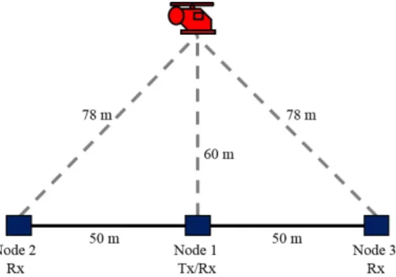
Fig. 1: Sketch of the experimental setup

MHz bandwidth, 0.6 µs pulse duration, 23 dBm transmitted power, and 5 kHz Pulse Repetition Frequency (PRF) to ensure that the whole UAV micro-Doppler signature is included in the unambiguous region. Horizontally polarized antennas with 10 degrees beam-width in elevation and azimuth and 24 dBi gain were used. This experiment was performed in July 2015 in an open field at the UCL Sports Grounds in Shenley, in collaboration with Fraunhofer FKIE. Fig. 1 shows a sketch of the experimental setup, with three NetRAD nodes deployed along a linear baseline with 50 m inter-node separation. Node 1 was used as monostatic transceiver, with node 2 and node 3 used as bistatic receiver-only nodes. The small UAV used in this experiment was the quadcopter DJI Phantom Vision 2+, performing different movements in an area at a distance from the baseline of 60 m or larger.

An example of a range-time-intensity (RTI) plot from NetRAD data is shown in Fig. 2. The small UAV signature can be seen between range bin 20 and 40. In this case the UAV was performing small movements, remaining mostly in the same range bin or moving across a limited number of range bins.

Fig. 2: Example of RTI NetRAD data

III. UAV DETECTION

This section describes the UAV detection and measurement generation process, which feeds the tracker that is described in the following section.

0 20 40 60 80 100 120 140 Range bin 0 200 400 600 800 1000 Signal strength Target Clutter (Trees)

Power per Cell Estimated Power Level Threshold

Fig. 3: Example of CFAR process

A. Constant False Alarm Rate Detector

A standard Constant False Alarm Rate (CFAR) detector was applied in range to generate target detections for each bistatic pair. A coherent processing interval (CPI) of 1000 pulses was used, as the pulse repetition interval was 5kHz, this resulted in five CPIs per second. For each range bin, the estimated clutter plus noise power level was determined by averaging over 10 adjacent cells, with one guard cell. An example of a single CPI is shown in Fig. 3.

Based on the estimated clutter plus noise power level ¯z, a thresholdT was applied:

T = ¯z·a (1) where: a=n·P− 1 n F −1.0 (2) n is the number of cells (in this case 20) and PF is the

probability of false alarm, taken as PF = 0.1. A detection is

declared for a range cell if the cell power exceeds the threshold as well as the power in adjacent guard cells.

After declaring a detection, the bistatic range is estimated by centroiding over adjacent range cells. The estimated range r is: rd= 2 X i=−2 rc(d+i)·z(d+i)2 (3)

whererc(x)is the range at the center of range binx,z(x)is

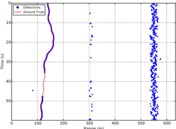
the voltage in range cell x and d the range cell for which the detection was declared. An example of the centroided detections after the CFAR is shown in Fig. 4. Calibration of the measurements was performed based on the measured GPS ground truth, to avoid GPS inaccuracies influencing the evaluation.

B. Micro-Doppler Discrimination

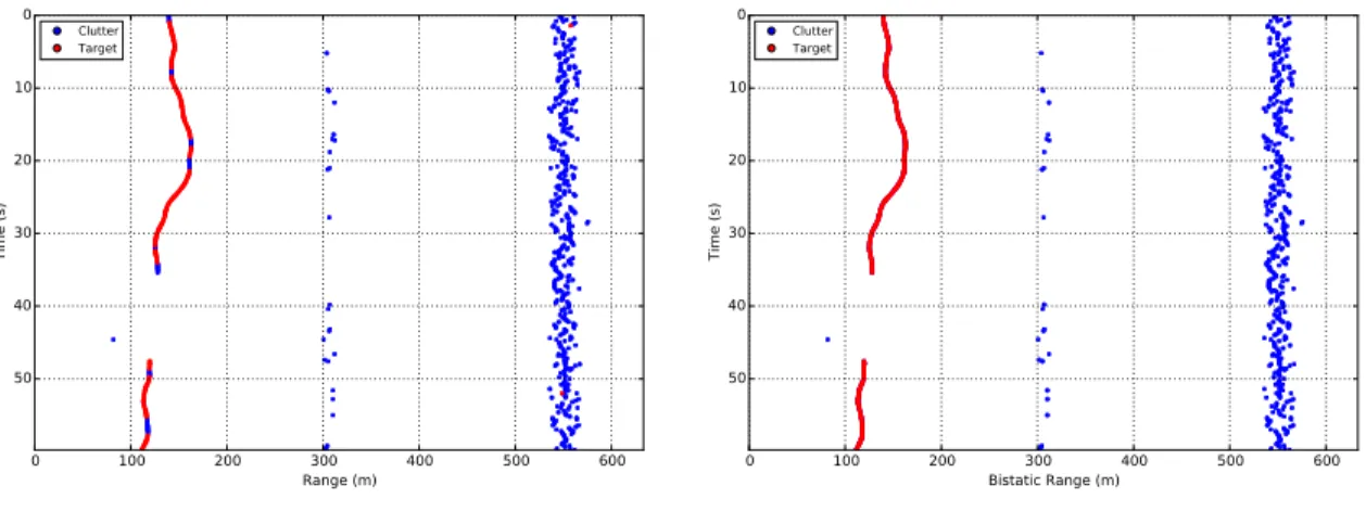
Moving targets can be discriminated from clutter returns based on the measured Doppler shift, when the radial velocity of the target of interest is substantially greater than the radial velocities of the clutter. However, a UAV can rapidly change velocity and also hover, making it difficult to separate from the clutter based on the Doppler shift alone. Fig. 5a shows the detections after the CFAR. Detections in the clutter notch are displayed in blue, and the moving target detections that are not

0 100 200 300 400 500 600 Range (m) 0 10 20 30 40 50 Time (s) Detections Ground Truth

Fig. 4: Centroided detections after CFAR detector.

in the clutter notch in red. It can be seen that UAV detections are lost when the UAV radial velocity is low, and some clutter detections are falsely considered to be a moving target.

In Fig. 6 the Doppler spectrogram of the clutter and of the UAV is illustrated. It can be seen that the signature of the clutter is very narrow in Doppler as the clutter is mostly stationary, whereas the UAV presents a significantly wider micro-Doppler signature because of the fast rotation of the blades. This characteristic can be used to improve the discrimination between the UAV and the clutter, as the blade rotation signature is present even when the UAV is hovering or moving with a reduced radial velocity, hence not presenting a significant main Doppler shift.

0.0 0.2 0.4 0.6 0.8 1.0 Time (s) 300 200 100 0 100 200 300 Radial velocity m/s

Spectrum of Range Bin 105 at time 1.0s

120 105 90 75 60 45 30 15 (a) Clutter 0.0 0.2 0.4 0.6 0.8 1.0 Time (s) 300 200 100 0 100 200 300 Radial velocity m/s

Spectrum of Range Bin 34 at time 1.0s

120 105 90 75 60 45 30 15 (b) UAV Fig. 6: Doppler spectrum of clutter and UAV.

To exploit the micro-Doppler for discriminating between clutter and the UAV, we apply the following procedure to each range bin for which the CFAR returns a detection:

1) The spectrum of the response is computed with the Short-time-fourier-transformation

2) The cell with the highest intensity pmax is found.

This corresponds to the main Doppler response 3) All cells with an intensity higher thanpmax−30dB,

which are more than 30m/s distant from the main Doppler are counted

4) If this number is higher than a threshold, a UAV detection is declared

Basically this procedure tests, whether the spectrum cor-responds to a peak centered around the main doppler or whether it is more spread out. Fig. 5b shows the results of this

procedure. Detections classified as clutter are shown in blue, and UAV detections in red. It can be seen that detections are no longer lost when the UAV radial velocity is low. Additionally, there are no longer detections generated by clutter that are thought to be UAV detections.

IV. UAV TRACKING

A measurement generated by a single bistatic pair provides the target bistatic range without any angle information. There-fore, although the UAV is detected it is not localised, as the bistatic range can refer to a set of locations on the oval of Cassini. To accurately estimate the position of the UAV, it is necessary to track the UAV, fusing the measurements from the different bistatic paths over multiple time steps. This section describes a tracking procedure using an extended Kalman filter. The target state at time k is assumed to be a two dimen-sional Cartesian vector:

xk = (x, y, x0, y0) (4)

and the position components of the target state are denoted

xp_k = (x, y). The tracker produces an estimate of this target state, denoted xˆk = (ˆx,y,ˆ xˆ0,yˆ0), with position components

denoted xˆp_k = (ˆx,yˆ). The filter predicted error covariance in the target state estimate at time k based on all measurement up to time kis denotedPk|k, the predicted covariance at time

k+ 1 given measurements up to timek is denotedPk+1|k.

Each bistatic pair produces a measurement of the bistatic range r corrupted by noise according to the measurement equation:

r=h(xk) +w (5)

where w is a measurement noise sequence with variance σr.

In this work σr is taken as 1m. In theory the measurement

noise standard deviation depends on the signal to noise ratio and the range resolution [11]. However, 1m is taken in this work as there are additional sources of error, such as the error arising from assuming a two dimensional target state when the UAV actually moves in three dimensions. The non-linear measurement function is:

h(xk) =kxr−x p

kk+kxt−x p

kk (6)

where xr= (xr, yr) is the position of the receiver andxt= (xt, yt)is the position of the sender.

The extended Kalman filter performs a linearisation of the non-linear measurement function based on the target state estimate ˆxk, to give the measurement matrix for a single

transmitter receiver pair:

Hk= (h0 h1 0 0) (7) where: h0= xˆ−xr ||xr−x p k|| + xˆ−xt ||xt−x p k|| (8) and h1= yˆ−yr ||xr−xp_k|| + yˆ−yt ||xt−xp_k|| (9)

It is assumed that there is just one target in the surveillance region and a track is initialized when measurements from at least two nodes are available. The track is initialized by

0 100 200 300 400 500 600 Range (m) 0 10 20 30 40 50 Time (s) Clutter Target

(a) Clutter notch equivalent to±0.5m/s.

0 100 200 300 400 500 600 Bistatic Range (m) 0 10 20 30 40 50 Time (s) Clutter Target

(b) Discrimination based on Micro-Doppler. Fig. 5: Detections classified as clutter (blue) and detections considered to be from UAV (red).

performing a least squares minimization, taking into account all available measurements of this time instance. If there are only two measurements available, the result is equal to the intersection of the corresponding ovals of Cassini.

The target motion is modelled with a linear state transition function:

xk+1=F·xk+v (10)

where v is a process noise sequence with covariance Q and the transition matrix Fis:

F=    1 0 t 0 0 1 0 t 0 0 1 0 0 0 0 1    (11)

where t is the time interval between measurements, which is the coherent processing interval time. A continuous white noise acceleration motion model [12] is assumed and therefore:

Q=     1 3·t 3 1 2·t 2 _{0 0} 1 2·t 2 _{t 0 0} 0 0 1₃·t3 1 2·t 2 0 0 1₂·t2 t     q (12)

as the UAV is highly manoeuvrable, the process noise q is taken as 100m2_/s3_.

Between time steps (coherent processing intervals) the target state estimate is predicted according to:

ˆ

xk+1=F·xˆk (13)

and the filter predicted error covariance is predicted according to:

Pk+1|k =FPk|kFT (14)

After each coherent processing interval, a maximum of three measurements may be available, originating from each of the bistatic pairs. These measurements are sequentially filtered into the state estimate based on the Kalman filter update equation:

ˆ

xk+1|k+1= ˆxk+1|k+K·(r−h(xk+1)) (15)

where xˆk+1 is the target state estimate at time step k+ 1, either predicted from the previous time step or after filtering the measurement from a different bistatic pair. The Kalman weight is:

K=Pk+1HTk+1S

−1 ₍₁₆₎

whereS is expected innovation variance:

S=Hk+1Pk+1|kHTk+1+R (17) The track covariance is updated according to:

Pk+1|k+1= (I−KHk+1)·Pk+1|k (18)

A track is dropped when the filter predicted covariance exceeds an expected RMSE of 30m, that isqtr(Pp_k|k)where

Pp_k|k is the covariance of the position components. V. RESULTS

The experiments consisted of a number of trials, with a ”DJI Phantom Vision 2+” target following a variety of trajectories. The UAV ground truth was captured using GPS devices.

Figure 7 shows the first scenario. The drone performed a flight along the main transmit beam and during this movement also moved down and up. It can be seen that the target is tracked with an RMSE around 0.5m to2.5m. A single track loss at time ∼ 39s appears as the UAV is on the near end towards the radar, which happens because it leaves the beam in altitude. Due to the up and down movement of the UAV perpendicular to the main movement, it regularly leaves the beam. In the other cases the loss is short enough for the tracker to recover. The two peaks in the RMSE at ∼13sand

∼58s, correspond to slightly longer times outside of the beam, although not long enough for an actual track loss. These two peaks occur, as the UAV is at the far side of its trajectory. At time ∼39s the UAV leaves the beam for a longer time and the track is dropped.

The second scenario is illustrated in Fig. 8. As with the previous scenario it can be seen that the UAV is accurately

0 20 40 60 80 100 120 140 x pos (m) +6.878e5 60 80 100 120 140 160 180 y pos (m) +5.7325e6 Rx 1 Rx 2 Rx 3 TX Start Position Ground Truth Track Tx beam Rx beam (a) Track 0 10 20 30 40 50 60 time (s) 0.0 0.5 1.0 1.5 2.0 2.5 3.0 3.5 RMSE (m) RMSE

(b) Root Mean Squared Error Fig. 7: Track and root mean squared error for trajectory 1.

tracked in the region where the transmit and receive beams overlap. Outside of this region, the error increases significantly and track drops can occur. It can be seen that in the time the UAV is tracked the RMSE is around 0.5m−1.5m. However when the UAV leaves the beam the RMSE rapidly increases. This is because without measurements the tracker predicts a linear movement, while the UAV performs a circular motion. The results of the third scenario are illustrated in Fig. 7. In Fig. 7a it can be seen that the resulting track very accurately follows the ground truth. In this scenario the target performs several small maneuvers, which are accurately followed by the tracker. It can also be seen that a track loss occurs as the UAV leaves the transmit beam. Fig. 7b plots the root mean squared error for the trajectory. Although for each bistatic pair no angle information is available, it can be seen that by fusing the multiple bistatic paths the UAV can be accurately tracked down to an RMSE of 0.5m to 1.5m.

VI. DISCUSSION ANDEXTENSIONS

In the results it was shown that by tracking with mea-surements from multiple bistatic pairs a small UAV can be very accurately tracked even though no angle information was available. However accurate tracking can only be performed in the intersection of the transmit and at least one additional receive beam. In the existing setup this amounted to a fairly restricted surveillance area. To track UAVs over a wider surveillance area antennas with a broader transmit and receive beam can be utilised. Another option would be to sweep the beams in a synchronised manner over the surveillance area. A mono-static detection then could adapively cue the passive receivers for accurate tracking.

This work can be extended in a number of ways. Firstly, the single target tracking approach applied in this work could be extended for multiple targets. This would be an increase in complexity, as ghost target hypotheses would need to be resolved. Additionally, the UAV detection could be extended to differentiate between human and UAV micro-Doppler. The target state was taken in two dimensions, however, the target could be tracked in three dimensions, as three bistatic range measurements are available.

VII. CONCLUSION

In this paper an approach for detecting and tracking a small UAV using experimental data colleced with the multistatic radar NetRAD was presented. In the detection stage, the UAV micro-Doppler signature was used to help discriminate between clutter returns and returns from the UAV. Using the micro-Doppler signatures was particularly beneficial in cases when the UAV radial velocity was very low, such as when the UAV hovers. By tracking the UAV using measurements generated from multiple bistatic pairs, it was possible to achieve a low RMSE, despite the lack of angle information.

REFERENCES

[1] M. Ritchie, F. Fioranelli, and H. Borrion, “Micro UAV Crime Pre-vention: Can we help Princess Leia?” in Preventing Crime Problems around the Globe through Research Innovations in the 21stCentury, B. L. Savona and E., Eds., TBA.

[2] K. Chetty, G. E. Smith, and K. Woodbridge, “Through-the-wall sensing of personnel using passive bistatic wifi radar at standoff distances,”

IEEE Transactions on Geoscience and Remote Sensing, vol. 50, no. 4, pp. 1218–1226, 2012.

[3] N. Mohajerin, J. Histon, R. Dizaji, and S. L. Waslander, “Feature extraction and radar track classification for detecting UAVs in civillian airspace,” in 2014 IEEE Radar Conference. IEEE, may 2014, pp. 0674–0679.

[4] R. I. A. Harmanny, J. J. M. de Wit, and G. P. Cabic, “Radar micro-Doppler feature extraction using the spectrogram and the cepstrogram,”

2014 11th European Radar Conference, pp. 165–168, 2014.

[5] J. J. M. de Wit, R. I. A. Harmanny, and P. Molchanov, “Radar micro-Doppler feature extraction using the Singular Value Decomposition,” in

2014 International Radar Conference. IEEE, oct 2014, pp. 1–6. [6] P. Molchanov, R. I. A. Harmanny, J. J. M. de Wit, K. Egiazarian,

and J. Astola, “Classification of small UAVs and birds by micro-Doppler signatures,”International Journal of Microwave and Wireless Technologies, vol. 6, no. 3-4, pp. 435–444, 2014.

[7] M. Ritchie, F. Fioranelli, H. Borrion, and H. Griffiths, “Classification of loaded/unloaded micro-drones using multistatic radar,” Electronics Letters, vol. 51, no. 22, pp. 1813–1815, 2015.

[8] M. Ritchie, F. Fioranelli, H. Griffiths, and B. Torvik, “Micro-drone RCS Analysis,” in2015 IEEE Radar Conference, 2015.

[9] D. Tahmoush, “Detection of small UAV helicopters using micro-Doppler,” inRadar Sensor Technology XVIII, K. I. Ranney and A. Do-erry, Eds., vol. 9077, Baltimore, Maryland, USA, may 2014.

0 20 40 60 80 100 120 140 x pos (m) +6.878e5 60 80 100 120 140 160 180 y pos (m) +5.7325e6 Rx 1 Rx 2 Rx 3 TX Start Position Ground Truth Track Tx beam Rx beam (a) Track 0 10 20 30 40 50 60 time (s) 0 1 2 3 4 5 6 7 8 RMSE (m) RMSE

(b) Root Mean Squared Error Fig. 8: Track and root mean squared error for trajectory 2.

0 20 40 60 80 100 120 140 x pos (m) +6.878e5 60 80 100 120 140 160 180 y pos (m) +5.7325e6 Rx 1 Rx 2 Rx 3 TX Start Position Ground Truth Track Tx beam Rx beam (a) Track 0 10 20 30 40 50 60 time (s) 0.0 0.5 1.0 1.5 2.0 2.5 3.0 RMSE (m) RMSE

(b) Root Mean Squared Error Fig. 9: Track and root mean squared error for trajectory 3.

[10] T. Derham, S. Doughty, K. Woodbridge, and C. Baker, “Modified input estimation technique for tracking manoeuvring targets,” Radar Sonar navigation IET, vol. 3, no. 1, pp. 30–41, 2007.

[11] D. K. Barton,Radar System Analysis and Modelling. Artech House Publishers, 2004.

[12] Y. Bar-Shalom, X. Rong Li, and T. Kirubarajan, Estimation with Applications to Tracking and Navigation:, 2001.