S. Suard, L. Audouin, F. Babik, L. Rigollet, J.C. Latch´e
Institut de Radioprotection et de Sˆuret´e Nucl´eaire (IRSN) Direction de la Pr´evention des Accidents Majeurs (DPAM)
BP 3 – 13115 St. Paul-lez-Durance, France
{sylvain.suard, laurent.audouin, fabrice.babik, laurence.rigollet, jean-claude.latche}@irsn.fr
Abstract
Fire is a major concern for the nuclear safety due to potential severe consequences of an uncontrolled fire on the surroundings of a nuclear plant. Since more a twenty years, a research program addressing this topic is in progress at the french ”Institut de Radioprotection et de Sˆuret´e Nucl´eaire” (IRSN). Within this framework, a computational code, named ISIS, dedicated to the simulation of buoyant fire in a compartment mechanically ventilated, is developed.
Physical models of this code are based on the Reynolds-Averaged Navier-Stokes equations, supplemented by a two-equation closure for turbulent flows and the eddy viscosity model. The turbulent production term is adapted to cope with buoyancy effects. Combustion modeling relies on classical eddy dissipation approaches and the flux-method is employed to treat radiation exchanges. Both incompressible and low Mach number flows are dealt with. For the numerical solution, a fractional step algorithm has been developed. To ensure stability and positivity of the discrete operators, the spatial discretization combines mixed finite element for the Navier-Stokes equations and finite volumes scheme for transport (advection-diffusion-reaction) equations.
For the verification of the code, a wide range of techniques is employed: comparison to analytical solution for model problems, use of manu-factured solution and comparison to benchmark result. We detail in this paper particular application of each kind; in all cases, convergence properties of the scheme are assessed.
Validation is now underway, and is based on the so-called building-block approach. We shortly describe some of the obtained results, first for an unit problem and then for a large-scale realistic experiment.
Key words : verification, validation, computational fluid dynamics, fire simulation
1
Introduction
The use of computational engineering, and in particular computational fluid dynam-ics, nowadays increasingly widespreads, a fundamental reason for this matter of fact being that the capacities of the computers currently allow to simulate large scale and complex systems evolving in time. In particular, safety studies addressing fire propagation in a nuclear plant, a tunnel or a shopping center use more and more simulation tools. This in turn motivates considerable research efforts in complex phenomena modelling, to evenly increase the field of investigation of computational applications.
In view of this central role played by computer predictions, a major questions rises, namely the assessment of the reliability of the simulations. More precisely, the problem posed is how to assess the degree of accuracy and validity of results given by a computer code; this is the aim of the verification and validation process (V&V). The Defense Modeling and Simulation Office (DMSO) of Department of Defense (DoD), [5, 6, 7] were the leaders in the development of concepts and terminology used in V&V. Nowadays, the most commonly referenced and agreed literature on this topic is probably the work of Roache [20], of Oberkampfet al. [16] and the AIAA guide [17]. Other works on verification and validation can be found in [2, 21, 22, 23]. Among the concepts clarification brought by these authors, the most important may be the following basic definition for verification and validation:
- Verification: the process of determining that a model implementation
accu-rately represents the developer’s conceptual model and the solution of the model.
- Validation: the process of determining the degree to which a model is an
accurate representation of the real world from the perspective of intended uses of the model.
The verification and the validation of the ISIS CFD code are presented in this pa-per, closely following the terminology introduced above. In the first two sections, we briefly describe the numerics and physics of this simulation tool, then we give in the two last sections examples of the verification and validation work up to now per-formed. For the verification step, three tests are presented, which roughly cover the range of techniques developed to this purpose: comparison to analytical solutions, use of manufactured solutions and comparison to benchmark results. Concerning validation, two cases are described: a simple unit problem, then the simulation of an experiment addressing the fire behavior in a large-scale compartment of a nuclear power plant.
2
Numerical Methods
We address in this section the numerical solution of the following class of problems:
∂ρ ∂t +∇ ·ρv= 0 (1a) ∂ρv ∂t +∇ ·(ρv⊗v) =−∇p+∇ ·τ + (ρ−ρ0)g (1b) ∂ρφ ∂t +∇ ·ρvφ=∇ · µe σφ ∇φ +Sφ (1c) ρ=G(φ,· · ·) (1d)
wheretstands for the time, vfor the fluid velocity, pfor the dynamic pressure, and
ρfor the fluid density. The tensor τ represents either the viscous stress tensor or in
turbulent regime, the Reynolds stress tensor. The density is supposed to be given explicitly as a function of the unknown fieldφ, and the volumic diffusion coefficient
µe/σφis strictly positive. The parameterσφstands, here, for a Prandtl or a Schmidt number. The problem is supposed to be posed over Ω, an open bounded connected subset ofRd withd= 2 or d= 3. It must be supplemented by initial and boundary conditions forvand φ.
Several physical problems enter this abstract framework. For instance, taking forφ
the temperature and forG(·) the equation of state of perfect gases evaluated at a fixed pressure yield the asymptotic governing equations of natural convection flows in the low Mach number limit. Withφequal to a concentration and a simple mixing rule to evaluate the density, we recover the system of equation modelling solutal convection of liquids. Last but not least, a model for the computation of diffusion flames is obtained when consideringφ as a Zeldovitch’s variable. The expression of G(·) can then be derived by calculating the temperature and the concentrations of the components as a function of φ and using the mixture equation of state. This computation yields the density value provided that the pressure used in the equation of state can be considered as constant,i.e. provided that we address once again low Mach number flows. In fact, this system can be viewed as central for the ISIS code, in the sense that the more complex models considered in practical applications can be obtained by complementing the system (1) by transport equations, the numerical solution of which closely follows the ideas developed for equation (1c) described hereafter.
To design a numerical scheme for the solution of system (1), one is faced to at least two difficulties. First, the unknownφcan be expected, from both physical and mathematical reasons, to meet L∞
and L2stability properties. This suggests to build
a finite volume numerical scheme which reproduces these features at the discrete level. Second, as the density of the fluid can be a function of the variable φ, the model at hand shares the mathematical properties of incompressible flow problems: no independent evolution equation can be stated for the fluid density; instead, the mass balance equation rather seems to act as a constraint on the velocity field which determines the pressure. This justifies the use of fractional step schemes issued from ISO/TC 92/SC4 Workshop on Assessment of Calculation Methods in FSE 3
the incompressible flow numerics, namely (extension of) projection methods, based
oninf-supstable pairs of velocity and pressure approximation spaces. Among these
last, nonconforming velocity approximations with degrees of freedom located at the center of the faces seem to be well suited to a coupling with a finite volume method for the advection-diffusion-reaction ofφ. A fractional step schemes relying on these basic ingredients, namely finite volumes for the computation ofφand finite element projection scheme for the solution of the momentum and mass balance equation, is presented below.
From a physical point of view, it seems natural for the fieldφto satisfy a maximum principle (for instance, both a concentration and a Zeldovitch’s variable must remain in the [0,1] interval). However, as the velocity field v is not divergence free, this is not a direct consequence of equation (1c), but of the system (1a)-(1c). More precisely, for any given regular velocity fieldv, a solution (ρ, φ) of (1a)-(1c), with a positive initial condition for ρ and an initial condition for φ taking values in [0,1], takes its values inR?+×[0,1]. The purpose of the developments presented hereafter
is to design a numerical scheme which enjoys the same properties. The central role played by the mass balance relation in both cases suggests the following three-step implicit Euler algorithm:
˜ ρ−ρn ∆t +∇U·ρ˜v= 0 (2a) ˜ ρφn+1−ρφn ∆t +∇U·ρφ˜ n+1 v−∆Cφn+1=Sφn+1 (2b) ρn+1=G(φn+1,· · ·) (2c)
where the preceding relations must be understood in the fully discrete sense, with the standard finite volume discretization for the time derivative term, ∇U·(·) stands
for the upwind (with respect to the velocity) finite volume discretization of the divergence operator and ∆C(·) is the usual centered discretization of the diffusion
terms (see [8] for a precise definition).
The first step of this algorithm is a prediction of the density, Eq. (2a). One has to note, in particular, that in view of the global algorithm, this evaluation of ˜ρ differs from a second order Richardson’s extrapolation only by the implicitation of ρ and the upwinding of the divergence term.
A numerical scheme for the solution of the full system of equations is simply ob-tained by complementing equations (2a)-(2c) by an incremental projection method. Writing this algorithm in a time-semidiscrete setting, this yields the following five
step scheme: solve for ˜ρ ρ˜−ρ n ∆t +∇U·ρ˜v n= 0 (3a) solve forφn+1 ρφ˜ n+1−ρnφn ∆t +∇U·ρφ˜ n+1 vn−∆Cφn+1=Sφn+1 (3b) ρn+1 given by ρn+1=G(φn+1,· · ·) (3c) solve for ˜v ρ˜v˜−ρ nvn ∆t +∇ ·(˜ρv n⊗v˜)− ∇ ·τ(˜v) +∇pn= 0 (3d) solve forpn+1, vn+1 ρn+1vn+1−ρ˜v˜ ∆t +∇(p n+1 −pn) = 0 ∇ ·ρn+1vn+1=−ρ n+1−ρn ∆t (3e)
The momentum and mass balance equations are discretized by a mixed finite ele-ment method based on a structured grid, using the so-called rotated bilinear eleele-ment for each velocity component and a piecewise constant pressure. The stability of this element is proven in [18]. The implementation of projection methods for incom-pressible flows, in particular with this element, is discussed in [24]. An extension of the projection method to dilatable flows is presented in [12, 4]. It is to note that the generalization of the scheme presented here to unstructured simplicial triangulations appears to be straightforward, as the used finite volume method handle this type of meshings and the rotated bilinear element can be replaced by the Crouzeix-Raviart one [9, p.132].
For the discretization of the time derivative in the velocity prediction and projection step, we use the standard trick which consists in lumping the mass matrix, i.e.
adding the contribution of the extra-diagonal terms of the diagonal and setting them to zero. As a consequence, the discrete counterpart of the first equation of (3e) yields directly un+1 and substituting the obtained expression in the second
relation yields a Poisson discrete problem for the pressure.
An upwind finite element discretization for the advective terms in equation (3d) is implemented using the flux correction tools presented in [13].
As the approximate pressure and density are constant over each element, the dis-cretization of the second relation of (3e) yields the same algebraic relation as a centered finite volume discretization, which can be written:
ρn+1−ρn
∆t +∇C·ρ
n+1
vn+1= 0 (4)
Since the density is updated after the computation of zn+1, this scheme does not
conserve the quantityρz. The conservativity property can be recovered, at the cost of loosing the propertyρn+1=G(zn+1), by solving once again the balance equation
forzat the end of the time step; these schemes are described in [1].
3
Physical Modelling
The basic model of the ISIS code relies on a low Mach number formulation of the Navier-Stokes equations, which is justified by the fact that buoyant fires are unani-ISO/TC 92/SC4 Workshop on Assessment of Calculation Methods in FSE 5
mously described as low-speed flows. This model is obtained by formally developping the compressible Navier-Stokes equations as a function of the Mach numberM and making M tends to zero. This process splits the pressure in a quantity constant with respect to the space variables, termed the thermodynamic pressure, and of order M−2
, and a variable part, named the hydrodynamic pressure, of order M0 ;
the fluid density then depends only on the thermodynamic pressure, which removes the compressibility effects on the flow.
The turbulence modelling, for variable density flow, is based on the Favre average or density-weighted average technique. Then the Boussinesq’s eddy viscosity concept is employed to model the turbulent transport, which allows to express the turbulent shear stress as a function of the mean velocity gradients and a turbulent viscosity, for which an additional modelling is required. The scalars fluxes are modelled by the gradient diffusion assumption with turbulent Prandtl or Schmidt number. In fine, a
k−εmodel is employed to predict the turbulent viscosity, in which the turbulence production term is modified to take into account buoyancy effects.
The turbulent combustion model, based on the conserved scalar approach, assumes a fast chemistry and relies on the eddy dissipation concept (EDC), which is an exten-sion of the eddy break up model (EBU), devoted to premixed turbulent combustion. Due to the wide range of physical problems addressed by the ISIS code, it is dif-ficult to go further in the description of the physical modelling in this section; in counterpart, we will provide a self-consistent presentation of each verification and validation case, including the set of solved conservation equations.
4
Verification tests
We present in this section three numerical verification tests; following the termi-nology of reference documents [11, 17], they assess consistency and convergence properties of the fractional step schemes and spatial approximation schemes above described. These verification tests are chosen to cover the range of available tech-niques developed to this purpose: first a comparison with an analytical solution, the so-called Taylor-Green vortices, then a manufactured solution of a natural con-vection problem under the Boussinesq hypothesis and, finally, a natural concon-vection benchmark problem in the low-Mach number regime.
For each case, we first give the set of governing equations, then we precise the numerical method and, finally, we present the observed convergence results.
4.1 A comparison to an analytical solution
Testing against analytical solutions, also called method of exact solutions, is per-haps the simplest mean to perform code verification. The major limitation of this technique is that governing equations admitting an analytical solution are usually obtained for physical problems much simpler than the real situation of interest, often leaving the physical phenomena uncoupled.
A - Problem description
This test case addresses on the two dimensional Taylor-Green vortices, which is a widely used benchmark problem for Navier-Stokes solvers verification. The com-putational domain is a unit square [0,1] x [0,1] and the set of partial differential equation considered here is:
∇ ·v= 0 (5a)
∂v
∂t +v· ∇v=−∇p+ν∆v (5b)
where ν is the kinematic viscosity, defined as the ratio of the viscous force to the inertial force. This parameter is constant in this test: ν= 0.01 m2/s.
This system admits the following analytical solution: v(x, y, t) =
−cos(πx) sin(πy) exp(−2π2νt) sin(2πx) cos(2πy) exp(−2π2νt)
p(x, y, t) = −0.25 [cos(2πx) + cos(2πy)] exp(−4π2νt)
provided that boundary and initial conditions are consistent with these expressions. We choose here to prescribe the velocity on the whole boundary of the computational domain.
B - Numerics
Uniform meshes are considered for this test case with resolutions of 10×10, 20×20, 40×40, 80×80 and 320×320. Numerical parameters and main features of the numerical scheme are gathered in the following table.
Initial and final time 0, 1
Time-step ∆t= 0.1/nwithn= 1,2,4,8,16,32
Solution algorithm semi-implicit fractional step scheme, obtained from equations (3d-3e) by settingρ= 1
Time discretization first (backward Euler) and second order (BDF 2) scheme Spatial discretization no discrete upwinding
C - Results
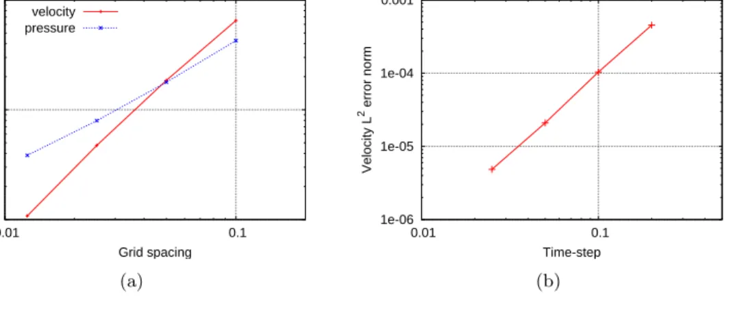
Spatial and temporal convergence for velocity and pressure are presented in Fig. 1 measured by theL2 error norm, defined as:
L2(φ) =
s Z
Ω
(S(x)−φh(x))2 (6)
where S(x) refers to the analytical solution and φh to the computational solution. Regarding, first, the spatial convergence, (Fig. 1a), theL2 norm of the error evolu-tion as a funcevolu-tion of the mesh step size for velocity and pressure are in agreement ISO/TC 92/SC4 Workshop on Assessment of Calculation Methods in FSE 7
with the theoretical results known for the considered spatial approximation scheme: second order convergence for the velocity, fist order one for the pressure. Temporal convergence is more difficult to check for the coarsest meshing because the spatial error is more important for this verification case than the temporal discretization error. With a 320×320 grid and the BDF2 time discretization, an order two time convergence is recovered, Fig. 1b.
0.001 0.01 0.1 0.01 0.1 L 2 error norm Grid spacing velocity pressure 1e-06 1e-05 1e-04 0.001 0.01 0.1 Velocity L 2 error norm Time-step (a) (b)
Figure 1: (a): Velocity and pressureL2 error norm vs. grid spacing; (b): VelocityL2 error norm
vs. the time-step.
4.2 An example of use of the manufactured solutions technique
The method of manufactured solutions is a more general approach for code verifi-cation. Owing to the fact that the principal disadvantage of the methods of exact solutions is to find an analytical solution to a given complex system of partial dif-ferential equations, an alternative consists in building an analytical source term by applying the considered partial derivation operators to a given solution. The man-ufactured solution is then the exact solution of the partial differential equations plus the analytical source terms. This method was first formalized by Roache and Steinberg [19] and a recent review is performed in [21]. A broad overview of code verification procedures based on the manufactured solution technique can also be found in [22].
A - Problem description
We address in this section a natural convection problem, within the Boussinesq assumption framework. In this test, the computational domain is the unit square and Navier-Stokes equation are supplemented by a balance energy equation:
∇ ·v= 0 (7a) ∂v ∂t + (v· ∇)v=−∇p+ 1 Re∇ 2 v+ Ra P rRe2θk+Sv (7b) ∂θ ∂t +v· ∇θ= 1 P rRe∇ 2 θ+Sθ (7c)
The unknown fields v, p and θ stand respectively for the dimensionless velocity vector, pressure and temperature and the parametersRe,RaandP rare respectively the Reynolds, Rayleigh and Prandtl numbers, which take the following constant values: Re= 100, Ra= 5000 and P r= 0.7. The vector k is the unit vector in the vertical direction.
A two-dimensional manufactured solution for the steady problem is derived from the 3D solution proposed in [3], by choosing the velocity, pressure and temperature as follows: v0 = [1−cos(2πx)] sin(2πz) sin(2πx)[cos(2πz)−1] p0 = sin(πx+π/2) sin(πz+π/2) θ0 = 1−z+x(1−x)z(1−z)
and building the source termsSv andSθ from the expression of (v0, p0, θ0): Sv= ∂v0 ∂t + (v0· ∇)v0− ∇p0− 1 Re∇ 2v 0− Ra P rRe2θ0k Sθ = ∂θ0 ∂t +v0· ∇θ0− 1 P rRe∇ 2 θ0
Boundary conditions (Dirichlet) are provided by the analytical manufactured solu-tion.
We suppose that the solution of the transient problem with these constant-in-time source terms and boundary condition tends toward the steady solution (v0, p0, θ0),
irrespectively of the initial condition, and we then arbitrarily set the initial velocity and temperature at zero: v(x, y) =θ(x, y) = 0.
B - Numerics
Uniform meshes are considered for this test case with resolutions of 10×10, 20×20, 40×40, 80×80 and 160×160. Numerical parameters and main features of the numerical scheme are gathered in the following table.
Initial time 0
Time step ∆t= 0.1
Final time
The computation is stopped when the L2 norm of the
difference between two consecutive time steps of both the velocity and the temperature, normalized by the
L2 norm of the solution, falls below<10−5 ∆t
Solution algorithm semi-implicit fractional step scheme, obtained from equations (3b, 3d-3e) by setting ρ= 1
Time discretization first order (backward Euler) scheme Spatial discretization
upwinding or hybrid approximation for the convective terms of the energy balance, no discrete upwinding for Navier-Stokes equations
C - Results
For the finite volume approximation of the temperature, we define the discreteL2
D error norm by:
L2D(φ) =
s Z
Ω
(Sh(x)−φh(x))2 (9)
where Sh(x) refers to the projection of the analytical solution in the finite volume discrete space (i.e. piecewise constant functions over each control volume) and φh to the computational solution.
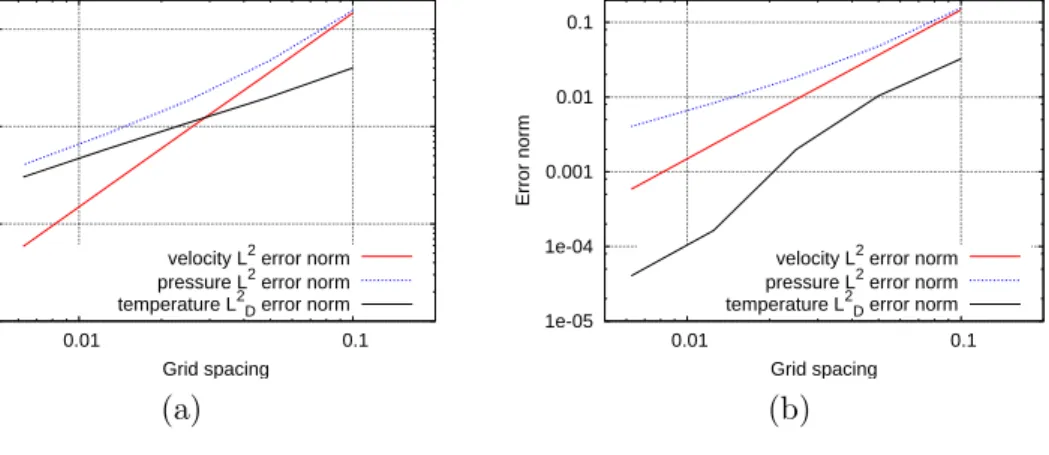
The behavior of the L2 error norm for velocity and pressure and of the discrete L2
error norm for temperature as a function of grid spacing is reported in Fig. 2, for the upwind (Fig. 2a) and hybrid (Fig. 2b) approximation of the convective terms in the energy balance.
With logarithmic scales, the upwind scheme exhibits a slope of unity (first order convergence) whereas the slope is two (second order convergence) for the hybrid approximation scheme. Results are thus in agreement with theoretical expectations, since formal convergence order is recovered.
1e-04 0.001 0.01 0.1 0.01 0.1 Error norm Grid spacing velocity L2 error norm pressure L2 error norm temperature L2D error norm
1e-05 1e-04 0.001 0.01 0.1 0.01 0.1 Error norm Grid spacing velocity L2 error norm pressure L2 error norm temperature L2D error norm
(a) (b)
Figure 2: Error norm for velocity, pressure and temperature. (a): upwind approximation scheme, (b): second order approximation scheme for the transport equation of the reduced temperature.
4.3 A comparison to a benchmark solution
Benchmark solutions are solution to physical problems which may be considered as accurate and reliable, because obtained and published by a wide panel of researchers using different and often high-performance numerical methods [17]. However, these verification tests, in most cases and up to now, are in two dimensions and essentially address laminar and incompressible flows.
A - Problem description
This test case is concerned with a differentially heated square cavity at high Rayleigh number with large temperature differences. Because of this last aspect, the
Boussi-nesq approximation is no longer valid and the use of a low Mach number formulation seems to be justified considering the low-level of the fluid velocity. Performances of the ISIS code in term of accuracy and grid convergence are compared to a reference solution recently given by Le Qu´er´e et al. [14]. The computational domain is a two-dimensional square enclosure [0,L]× [0,L], as sketched in Fig. 3. The left and right vertical walls are respectively heated toTh and cooled down to Tc, and a zero heat flux is imposed at the two horizontal walls. A no-slip condition is prescribed for the velocity fieldv.
g v= 0 v= 0 L Th v= 0 Tc v= 0
Figure 3: Configuration of thermally driven cavity.
The governing equations for this test case read:
∂ρ ∂t +∇ ·ρv= 0 (10a) ∂ρv ∂t +∇ ·(ρv⊗v) =−∇p+∇ ·τ + (ρ−ρ0)g (10b) ∂ρh ∂t +∇ ·ρvh = dPth dt +∇ · µ P r∇h (10c) ρ= Pth RT (10d)
wheretstands for the time,vfor the fluid velocity vector,pfor the dynamic pressure, and ρfor the fluid density. The tensor τ is the viscous part of the stress tensor for
a Newtonian fluid, given by the following expression:
τ =µ
∇v+∇tv−2
3(∇ ·v)I
The dynamic viscosityµfollows the Sutherland’s law:
µ(T) µ∗ = T T∗ 32 T∗ +S T +S where T∗ = 273 K, S = 110.5 K and µ∗ = 1.68 ×10⁻⁵ kg/(m.s). In the energy balance equation (10c), the enthalpy h is defined as h = cp(T −T0), with T0 a
reference temperature andcp the specific heat. The Prandtl number,P r, is assumed to remain constant with respect to the temperature and is defined as:
P r =cpµ(T) λ(T)
whereλ(T) is the thermal conductivity. In the low Mach approximation used here, the thermodynamic pressure, Pth, is constant in space and the dynamic part of pressure is neglected in the equation of state (10d). The mass conservation principle yields the following additional equation, which is used to compute the evolution of the thermodynamic pressure:
Pth(t) =m0 Z Ω 1 RT(x, t)dx
wherem0 is the initial mass.
This problem involves two main parameters, the Rayleigh numberRa and the tem-perature difference parameterεdefined by:
Ra=P rgρ 2 0(Th−Tc)L3 T0µ20 = 106 (11) and ε= Th−Tc Th+Tc = 0.6 (12)
where ρ0 = ρ(T0, P0) and µ0 = µ(T0) describe the density and shear viscosity at
a given reference temperature T0 and thermodynamic pressure P0. Heat transfers
to the hot and cold wall are represented by the local and average Nusselt numbers, respectively defined by:
N u(y) = L k0(Th−Tc) k∂T ∂x|w, N u= 1 L Z y=L y=0 N u(y)dy (13)
wherek is the thermal conductivity, defined by k(T) =cpµ(T)/P r, k0 =k(T0).
At steady-state and with the prescribed boundary conditions, integration of the energy equation over the volume of the square cavity implies that the average Nusselt numbers on the two vertical walls are equal:
N uh =N uc (14)
where subscriptsh and c refers to the hot and cold wall. The parameters of the simulation are:
- Gas constant: R= 287 J/(kg.K) - Ratio of specific heat: γ = 1.4
- Specific heat: cp =γR/(γ−1) J/(kg.K) - Prandtl number: P r= 0.71
- Gravity: gy =−9.81 m/s2
- Reference temperature: T0 = 600 K
- Reference pressure: P0= 101325 Pa
Spatially uniform initial conditions are imposed: ∀(x, y)∈[0, L]2, T(x, y) =T 0 and v(x, y) = 0. The prescribed temperature on vertical walls are Th =T0(1 +ε) and
B - Numerics
Various uniform grid size are used, obtained by successive refinements. Numerical parameters and main features of the numerical scheme are gathered in the following table.
Initial and final time 0 s, 50 s Time step ∆t= 0.05 s
Solution algorithm
semi-implicit fractional step scheme, obtained from equations (3a-3e), where the variable φ is to be understood as the temperature
Time discretization first order (backward Euler) scheme Spatial discretization
hybrid approximation for the convective terms of the energy balance, no discrete upwinding for Navier-Stokes equations
C - Results
One of the outputs of the benchmark was a reference value for the Nusselt number and the thermodynamic pressure at steady state, commonly agreed up to 5 digits:
N uh= 8.6866, P/P0 = 0.9244
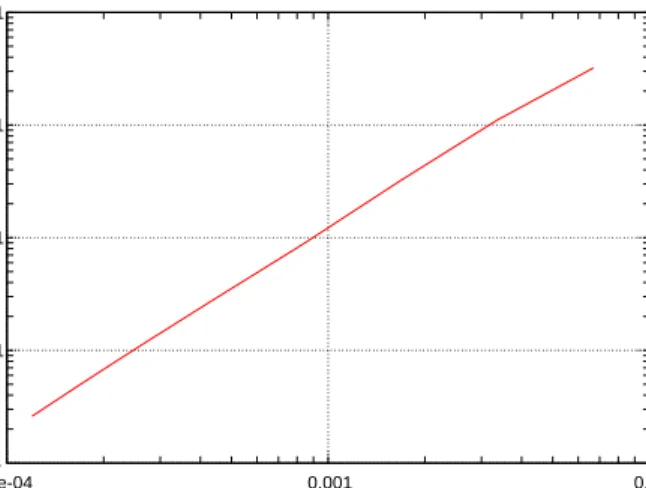
These results, obtained for different grid size, are reported in table 1 with the relative error between the computational solution and the reference solution. Fig. 4 shows an approximately second order convergence for the Nusselt number.
#dofs N uh EN uh Pth/P0 EPth/P0 1 600 8.4087 3.19e-2 0.9571 3.54e-2 6 400 8.6099 8.83e-3 0.9335 9.89e-3 25 600 8.6641 2.58e-3 0.9270 2.6e-3 57 600 8.6646 1.24e-3 0.9257 1.40e-3 102400 8.6801 7.39e-4 0.9251 8.64e-4 160 000 8.6783 4.89e-4 0.9249 5.99e-4 313 600 8.6822 2.59e-4 0.9247 3.60e-4
Table 1: Mean Nusselt number and thermodynamic pressure obtained with different grid sizes.
5
Validation tests
Validation is defined as the process of determining the degree to which a model is an accurate representation of the real world from the perspective of the intended
1.e-04 0.001 0.01 Grid spacing 1.e-04 0.001 0.01 0.1 1
Relative error on the mean Nusselt number
Figure 4: Relative error on the mean Nusselt number function of the grid spacing.
uses of the model in reference documents [11, 17]. Main concepts interacting in the
validation pocess are largely clarified in [17] and this discussion is far beyond the scope of the present paper. Instead, we focus here on the implementation of the so-called ”validation phases method” for the fire simulation ISIS code. This method, also called the building-block approach [17, 16], consists in breaking up the complex engineering system of interest in several sub-systems of less complexity. Generally speaking, this simplification process generates three levels of decreasing complexity: into the first class, corresponding to the highest level of complexity, fall the so-called ”sub-system cases”; the second class gathers ”benchmark cases” and the last one ”unit problems”. Simplification may consist of uncoupling physical phenomena, adressing steady state cases instead of transient ones, approximating boundary con-ditions by simpler ones, idealizing the geometry . . . For each sub-system, benchmark case and unit problem, code results will have to be compared to experimental data or published reliable solutions.
The validation process may include a calibration work, a definition of which can be found in [17, section 4.2]:
”Calibration: the process of adjusting numerical or physical modelling
param-eters in the computational model for the purpose of improving agreement with experimental data.”
For the particular topic of fire simulation, the main concerned physical models are the turbulence and reaction rate modelling. As far as possible, the calibration phase has to be gone through first, as any change in a basic modelling may make another iteration of at least a part of the validation process necessary.
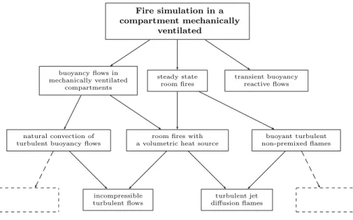
The validation process of the ISIS code has just begun at IRSN, and will be pursued over next years, together with the realization of supporting experimental programs. An example of what could be a building-block approach developed to this purpose is sketched on Fig. 5; of course, the choice of the different blocks of each three tiers is not unique. We restrict here the presentation to two validation works. The first
one falls in the class of unit problems; in the second one, we address a full-scale experimental fire in a compartment mechanically ventilated.
Fire simulation in a compartment mechanically ventilated buoyancy flows in mechanically ventilated compartments steady state room fires transient buoyancy reactive flows natural convection of turbulent buoyancy flows
room fires with a volumetric heat source
buoyant turbulent non-premixed flames incompressible turbulent flows turbulent jet diffusion flames
Figure 5: Validation phases
5.1 A unit problem
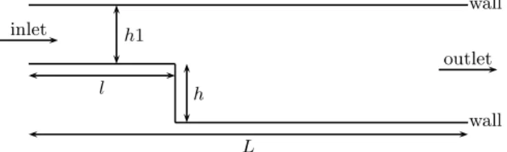
Turbulent flows over backward facing steps are widely used benchmark problems to evaluate the performance of turbulence models in the prediction of separated flows. This test focuses on the specific case of the incompressible flow over a backward-facing step at a Reynolds number of 44 500, based on the step height and the flow velocity uref just before the step. Under these conditions, the flow everywhere may be taken as fully turbulent.
A comparison of various commercial CFD code on this benchmark problem is de-scribed in [10], together with main experimental results. Code benchmarking sup-plements the code-to-experience comparison with respect to two aspects. First, the comparison between CFD codes allows to identify slight model variants (small change of parameters, different implementation of boundary conditions,...) which may be difficult to uncover in models presentations in the literature and codes doc-umentation, while strongly modify the results. In addition, provided that model identity can be checked, it yields an additional verification test (i.e. checking the correctness of the numerical solution of the model set of PDE).
A - Problem description
The computational domain is presented in Fig. 6.
wall inlet outlet h1 L l wall h
Figure 6: Backward facing step configuration. h= 3.8096 cm,L= 76.2 cm,l = 19.054 cm, and
h1 = 7.6204 cm.
The flow is governed by the following set of balance equations:
∇ ·v= 0 (15a) ∂ρv ∂t +∇ ·(ρv⊗v) =−∇p+∇ ·τ (15b) ∂ρk ∂t +∇ ·ρvk=∇ · µe σk ∇k +Gk−ρε (15c) ∂ρε ∂t +∇ ·ρvε=∇ · µe σε ∇ε + ε k(cε1,1Gk−cε2ρε) (15d)
where µe = µ+µt is the effective viscosity. The eddy viscosity model is used to express the turbulent viscosity as: µt =ρCµk2/and the Reynolds stress tensor,τ,
in the momentum equation is modelled with the Boussinesq hypothesis:
τ =µe ∇v+∇tv−2
3ρkI
The generation of turbulent kinetic energy results of the interaction of the turbulent shear stress and mean velocity gradients:
Gk=τ ⊗ ∇v
The model constants are set to the following standard values:
σk= 1., σε= 1.3, cµ= 0.09, cε1,1 = 1.44, cε2= 1.92
Fluid density and viscosity are respectively:
ρ= 1.0 kg/m3, µ= 1.101×10⁻⁵
kg/m/s.
Boundary conditions are set as follows:
- inlet : u= 13.m/s, v= 0, k= 0.7605 m2/s2, ε= 31.78 m2/s3.
- outlet: homogeneous Neumann condition foru, v, k, and ε. - all walls: turbulent wall functions.
B - Numerics
The steady state is approached by a transient computation, starting from the fol-lowing initial conditions:
v(x) = 0, k(x) = 0.01, and ε(x) = 0.01
Numerical parameters and main features of the numerical scheme are gathered in the following table.
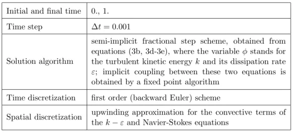
Initial and final time 0., 1.
Time step ∆t= 0.001
Solution algorithm
semi-implicit fractional step scheme, obtained from equations (3b, 3d-3e), where the variable φ stands for the turbulent kinetic energy k and its dissipation rate
ε; implicit coupling between these two equations is obtained by a fixed point algorithm
Time discretization first order (backward Euler) scheme
Spatial discretization upwinding approximation for the convective terms of thek−ε and Navier-Stokes equations
C - Results Velocity profiles
In Fig. 7 and Fig. 8, a good agreement can be observed between results obtained with the ISIS code and reference data (Ref represents average results obtained with SMARTFIRE, PHOENICS and CFX).
0 0.02 0.04 0.06 0.08 0.1 0.12 -4 -2 0 2 4 6 8 10 12 14 Y Displacement U Velocity ISIS Ref
Figure 7: Velocity profiles 0.285 m downstream of inlet.
0 0.02 0.04 0.06 0.08 0.1 0.12 0 2 4 6 8 10 12 Y Displacement U Velocity ISIS Ref
Figure 8: Velocity profiles at the outlet.
Reattachment length
The reattachment length is determined by locating the region where the stream-wise velocity component is changing from positive to negative (i.e., u =0.0) along the lower duct wall. Results of the benchmark [10] obtained with SMARTFIRE, PHOENICS and CFX are reported below, Table 2. S represents the reattachment length from the step. The reduced experimental value isS/h= 7.2.
Reat. length SMARTFIRE PHOENICS CFX ISIS
S 0.2217 0.2587 0.1967 0.2124
S/h 5.82 6.79 5.16 5.57
Table 2: Prediction of reattachment length for CFD codes
The code predicts the reattachment length with a relative error of 22.5 %. This is coherent with the fact that the standardk−ε model with wall functions is known to underpredict the reattachment length in the backward facing step by an amount in the order of 20-25 %.
5.2 A complex system
We address in this section the simulation of a real scale experimental fire [15]. This test has been performed at IRSN, as a part of an experimental program performed to provide data for the validation of computational tools simulating fires in mechan-ically ventilated compartments, with first application to nuclear power plant. This test turns out to be particularly difficult, for essentially two reasons. The first one is that the large scale geometry of the studied problem as well as the duration of the transient of interest make the computational requirements considerable; our first
concern will then be to assess the code stability and convergence for such systems. Second, the flow results from an intricate coupling between non-linear phenomena, as turbulence, combustion and buoyancy effects; separate validation of each single model will then be clearly out of reach, and we rely for this purpose on the previously described building-block approach. In the same direction, note in addition that the knowledge of initial and boundary conditions, together with the characterization of the flow are necessarily less comprehensive than in experiments carried out at the laboratory scale, which even reinforces the interest of validating each ”elementary” model using simpler experiments.
A - Problem description
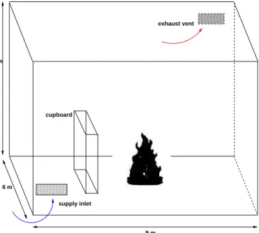
The experiment consists in a confined ethanol pool fire in a compartment mechan-ically ventilated with a metal cupboard close to the fire. The schematic diagram of the compartment fire is shown in Fig. 9. The dimensions are for the x, y and
z directions, respectively, Lx = 9 m, Ly = 6 m and Lz = 7.5 m. The different walls, the floor and the ceiling are 0.25 m thick concrete walls. The compartment is connected to a ventilation network including a forced ventilation supply inlet and a forced ventilation exhaust vent (Fig. 9) with respectively dimensions of 0.3 m2 and 0.4 m2. The ventilation rate is 5 h-1 and the depression -200 Pa. The pool fire is a
square of surface 1 m2 and height 0.13 m, located at the center of the compartment.
The fire heat release rate, defined as the product of the fuel mass loss rate and the heat of combustion of ethanol reaches 563 kW during the stationary combustion phase, Fig. 10. 6 m 9 m 7.5 m exhaust vent supply inlet cupboard
Figure 9: Experimental fire case geometry.
0 0.005 0.01 0.015 0.02 0.025 0.03 0 500 1000 1500 2000 2500
Fuel mass loss rate (kg/(s.m
2 )
Times (s)
Figure 10: Fuel mass loss rate in the experimental fire case.
The system describing the turbulent reactive flow in the low Mach number regime is presented below. The approximation turbulence resort to the mass-weighted averag-ing, also called the Favre averaging. A modifiedk−εmodel based on the Boussinesq hypothesis and the eddy viscosity model is used for turbulence closure. To model the turbulent combustion process, we use a fast chemistry assumption and the con-served scalar approach; we keep as unknowns variables the mixture fraction variable
z and the fuel mass fraction Yf. Removing for short in the notations the Favre or Reynolds turbulence averaging operators, governing equations read:
- mass balance: ∂ρ ∂t +∇ ·ρv= 0 - momentum balance: ∂ρv ∂t +∇ ·(ρv⊗v) =−∇p+∇ ·τ + (ρ−ρ0)g
- turbulent kinetic energy balance:
∂ρk ∂t +∇ ·ρvk =∇ · µe σk ∇k +Gk+Gb−ρε
- viscous dissipation balance:
∂ρε ∂t +∇ ·ρvε=∇ · µe σε ∇ε + ε k(cε1,1Gk+cε1,2Gb−cε2ρε) - enthalpy balance: ∂ρh ∂t +∇ ·ρvh=∇ · µe σh ∇h +dPth dt
- mixture fraction balance: ∂ρz ∂t +∇ ·ρvz=∇ · µe σz ∇z
- fuel mass fraction balance:
∂ρYF ∂t +∇ ·ρvYF =∇ · µe σYF ∇YF + ˙ωF
The Reynolds stress tensor, τ, appearing in the momentum equation, is expressed
as: τ =µe ∇u+∇tu− 2 3(∇ ·u)I −2 3ρkI Turbulent production terms are defined as:
Gk=τ ⊗ ∇v, Gb = µt ρσg
∇ρ·g
where the term Gb stands for the generation and destruction of turbulence due to buoyancy forces. In multicomponent mixtures, the density of the mixture is evaluated by: ρ= PthW RuT , with 1 W = N X k=1 Yk Wk
whereW is the mean molar weight of the mixture andYkandWkrespectively stand for the mass fraction and the atomic weight of species k (i.e. fuel, . . . ). The fuel burning rate is calculated according to:
˙ ωF =−CEBUρ kmin YF, YO s
whereCEBU is a model constant commonly taken of the order of four but which can be modelled by a viscous mixing model; here, we use the first option: CEBU = 4. To deal with radiative losses, we use the so-called Markstein model, so the specific enthalpy is linked to the temperature by the following relation:
h=cP(T−T0) + ∆Hc(1−χr)YF
where T0 is a reference temperature, ∆Hc is the heat of combustion and χr is the fraction of energy of combustion lost by radiative transfer; χr is set to 0.25 in this simulation. The model constants have the following standard values:
cµ= 0.09, cε1,1 = 1.44, cε2 = 1.92, cε1,2 = 1.44,
σk = 1., σε= 1.3, σh=σz =σYF = 0.71
The thermodynamic pressure of the room is computed by solving a simplified (0 D) momentum balance equation for the system composed of the confined compart-ment and the ventilation network. In this modelling, a Bernoulli general equation ISO/TC 92/SC4 Workshop on Assessment of Calculation Methods in FSE 21
describes each branchi of the network, which is, in this particular case, connected to the compartment: Li Si ∂Qi ∂t =Pth−Pnode,i−f
where Qi is the flow rate in the branch i, Pnode,i is the pressure at extremity of the branch which is not located at the compartment wall andf is an aerodynamic resistance. The geometrical dimensions Li and Si are respectively the length and the surface of the branchi. This system must be supplemented by the overall mass balance equation of the compartment:
Z Ω ∂ ∂t PthW RT +X i Qi= 0
Geometrical and material properties are gathered in the following tables. - gas mixture: dynamic viscosity µ= 1.68×10⁻⁵ kg/(m.s) thermal conductivity λ= 0.018 W/(m.K) specific heat cP = 1100 J/(kg.K) Prandtl number P r= 0.71 heat of combustion ∆Hc= 2.56×10⁷ J/kg - concrete walls: density ρw= 2430 kg/m3 thermal conductivity λw= 1.5 W/(m.K) specific heat cP,w = 736 J/(kg.K) walls thickness ew= 0.25 m - metal cupboard: density ρc= 7801 kg/m3 thermal conductivity λc= 43 W/(m.K) specific heat cP,c= 473 J/(kg.K) walls thickness ec= 0.25 m
Initial conditions are given by:
v=p=h=z=YF = 0,
k= 10−12
m2/s2, ε= 10−9
m2/s3, T = 290.K, ρ=ρair To define the boundary conditions, three different surfaces are considered:
- fire:
v= (0,0, wF), h= ∆Hc(1−χr), z=YF = 1, k= 0.1w2F, ε=Cµ
k3/2
lε wherewF is function of the fuel mass loss rate, wF = ˙mF/ρF and lε∼0.07L withLa characteristic length scale, equivalent to fire radius.
- walls: conduction in walls is accounted for in the energy balance equation. A log-law wall function is used for the momentum and turbulence balance equations.
- supply inlet and exhaust vent: a prescribed velocity is computed to match the flow rate in each branch; fuel is supposed to remain in the compartment. B - Numerics
Varous non-uniform grid are tested with 8 500, 68 000 and 240 000 meshes named thereafter mesh1, mesh2 and mesh3. Numerical parameters and main features of the numerical scheme are gathered in the following table.
Initial time 0., 1.
Final time 2800 s for mesh1, 1000 s for mesh2 and 250 s for mesh3 Time step ∆t= 0.1 s for mesh1 and mesh2, and 0.05 s for mesh3
Solution algorithm
semi-implicit fractional step scheme implemented for transport equations similar to (3e) for k, ε, h, z and
Yf variables; implicit coupling between the k −ε two equations and the two transport equations for z and
YF is obtained by a fixed point algorithm Time discretization first order (backward Euler) scheme
Spatial discretization upwinding approximation for the convective terms of thek−εand Navier-Stokes equations
C - Results
Thermodynamic pressure and mass flow rate
The evolution of the thermodynamic pressure in the compartment fire as a function of time (see Fig. 11) is in a good agreement with the experiment data. During the combustion stationary phase, the calculated pressure oscillates around -2 hPa and the amplitude of the oscillations is less strong than in the experiment. A strong overpressure at ignition and a weak depression at extinction are observed in both cases.
The evolution of mass flow rate at the supply inlet according to time is shown in Fig. 12. It stabilizes around 0.7 kg/s after a short period corresponding to the ignition phase. The mass flow rate at exit, not shown here, is almost identical. These results lie in the uncertainty range of the experimental data.
0 500 1000 1500 2000 Time (s) 0 -1 -2 -3 P th -P ref (hPa) ISIS Exp.
Figure 11: Thermodynamic pressure vs. time.
0 500 1000 1500 2000 2500 Time (s) 0.2 0.4 0.6 0.8
Mass flow rate (kg/s) ISIS
Exp.
Temperature in the plume region
The evolution of temperature with time in the plume region, 3 meters above the fire, obtained with mesh1 is presented in Fig. 13. for the whole transient and for the first 250 s in Fig. 14. After the time t = 250 s, both the computed and experimental temperature oscillate around similar values until the end of fire. The predicted peak of temperature in the early transient, not observed in experiments, could be due to the absence of models in the code to simulate combustion in the transition from the laminar to the turbulent flow regime, as occurs at ignition. Fig. 14 points out strong temporal variations of temperature corresponding to a rotation of the flame around its axis. This flame rotatory behavior is also observed in experiments with an almost equal frequency but with an amplitude of temperatures variations twice stronger. 0 500 1000 1500 2000 2500 Time (s) 0 250 500 750 1000 T-T 0 ISIS Exp.
Figure 13: Temperature vs. time to 3 meters above the fire.
As far as numeric are concerned, the code shows quite satisfactory stability prop-erties, allowing, in particular, the limitation of the time step to be based only on accuracy considerations. As expected, spatial convergence cannot be considered as achieved, even for the finer mesh; qualitative results however remain similar. Studies are ongoing to overcome this latter limitation, by extensive use of parallelism and development of more accurate spatial discretizations.
500 1000 1500 Time (s) 100 200 300 T-T 0 ISIS Exp.
Figure 14: Temperature vs. time to 3 meters above the fire.
6
Conclusion
We have presented in this paper some verification and validation tests of the ISIS CFD code, following the strategy recommended by the reference ISO document [11], DoD [6, 7], Roache [21] and the AIAA guide [17].
Three verification cases are presented, with the purpose of illustrating the main tech-niques developed for the purpose of code verification, i.e. comparison to analytical, manufactured and benchmark solutions.
The validation of the ISIS code is now underway, following the strategy of the so-called building-block approach. Two preliminary validation tests are presented. The first one falls in the class of unit tests problems, as the second one address a real-scale realistic experiment. The complexity of this last exercise clearly highlights the interest of the chosen progressive approach.
Acknowledgements
The practical implementation of the ISIS CFD code is based on the software object-oriented component library PELICANS, developed at IRSN. The authors would like to thank B. Piar and D. Vola for their support, in particular concerning the use of this computational platform, and for useful discussions. We also thank E. Garnier and M. Jobelin for their contributions to this work, in particular for the LIC1.14 validation case.
References
[1] F. Babik, T. Gallouet, J.-C. Latch´e, S. Suard, and D. Vola. On two fractional step finite volume and finite element schemes for reactive low Mach number flows. In The International Symposium on Finite Volumes for Complex
[2] I. Babuska and J.T. Oden. Verification and validation in computational engi-neering and science: basic concepts. Computer Methods in Applied Mechanics
and Engineering, 193(36-38):4057–4066, 2004.
[3] A. Benzaoui, X. Nicolas, and S. Xin. Efficient vectorized finite-difference method to solve the incompressible Navier-Stokes equations for 3-D mixed-convection flows in high-aspect-ratio channels. Numerical Heat Transfer, Part B, 48:277–302, 2005.
[4] X. Cor´e, P. Angot, and J. C. Latch´e. A multilevel local mesh refinement pro-jection method for low Mach number flows. Mathematics and Computers in
Simulation, 61:477–488, 2003.
[5] DoD. Dod directive no. 5000.59: Modeling and simulation (M&S) management. Defense Modeling and Simulation Office, Office of the Director of Defense Re-search and Engineering, 1996. available at: www.dmso.mil/public.
[6] DoD. Verification, Validation, and Accreditation (VV&A) - Recommended Practices Guide. Defense Modeling and Simulation Office, Office of the Director of Defense Research and Engineering, 1996. available at: www.dmso.mil/public. [7] DoD. Dod instruction 5000.61: Modeling and Simulation (M&S) - Verification, Validation, and Accreditation (VV&A). Defense Modeling and Simulation Of-fice, Office of the Director of Defense Research and Engineering, 2003. available at: www.dmso.mil/public.
[8] R. Eymard, T. Gallouet, and R. Herbin. The finite volume method. InHandbook
for Numerical Analysis. Ciarlet, P. and Lions, J.L., 2000.
[9] V. Girault and P.-A. Raviart. Finite Element Methods for Navier-Stokes
Equa-tions. Theory and Algorithms, volume 5 of Springer Series in Computational
Mathematics. Springer-Verlag, 1986.
[10] A.J. Grandison, E.R. Galea, and M.K. Patel. Fire modelling stan-dards/benchmark, report on phase 1 simulations. Technical report, Fire Safety Engineering Group, University of Greenwich, London SE10 9LS, 2001.
[11] ISO/TC 92. Fire safety engineering: Assessment, verification and validation of calculation methods. Technical report, ISO, 2005.
[12] O. M. Knio, H. N. Najm, and P. S. Wyckoff. A Semi-implicit Numerical Scheme for Reacting Flow: II. Stiff, Operator-Split Formulation. Journal of
Computa-tional Physics, 154:428–467, 1999.
[13] D. Kuzmin and M. Moller. Algebraic flux correction I. scalar conservation laws. Technical report 249, University of Dortmund, 2004.
[14] P. Le Qu´er´e, C. Weisman, H. Paill`ere, J. Vierendeels, E. Dick, R. Becker, M. Braack, and J. Locke. Modelling of natural convection flows with large temperature differences: A benchmark problem for low Mach number solvers.
Part 1. Reference solutions. Mathematical Modelling and Numerical Analysis, 39(3):609–616, May 2005.
[15] W. Le Saux. Essai LIC1.14 : r´esultats exp´erimentaux. Technical report, IRSN, 1997.
[16] W.L. Oberkampf, T.G. Trucano, and C. Hirsch. Verification, validation, and predictive capability in computational engineering and physics. InVerification and Validation for Modeling and Simulation in Computational Science and
En-gineering Applications, October 22-23 2002.
[17] American Institute of Aeronautics and Astronautics. Guide for the verification and validation of computational fluid dynamics simulations. Technical report, AIAA, 1998.
[18] R. Rannacher and S. Turek. Simple nonconforming quadrilateral Stokes ele-ment. Numerical Methods for Partial Differential Equations, 8:97–111, 1992. [19] P. J. Roache and S. Steinberg. Symbolic manipulation and computational fluid
dynamics. AIAA J., 22:1390–1394, 1984.
[20] P.J. Roache. Verification and Validation in Computational Science and
Engi-neering. Hermosa Publishers, 1998.
[21] P.J. Roache. Code Verification by the Method of Manufactured Solutions.
Journal of Fluids Engineering, 114:4–10, 2002.
[22] C.J. Roy. Review of code and solution verification procedures for computational simulation. Journal of Computational Physics, 205(1):131–156, 2005.
[23] F. Stern, R. Wilson, and J. Shao. Quantitative V&V of CFD simulations and certification of CFD codes. International Journal for Numerical Methods in
Fluids, 50(11):1335–1355, 2006.
[24] S. Turek. Efficient Solvers for Incompressible Flow Problems : An Algorithmic