UCLA Fall Quarter 2011-12
Electrical Engineering 103
Applied Numerical Computing
Professor L. Vandenberghe
Contents
I
Matrix theory
1
1 Vectors 3
1.1 Definitions and notation . . . 3
1.2 Zero and unit vectors . . . 4
1.3 Vector addition . . . 5
1.4 Scalar-vector multiplication . . . 6
1.5 Inner product . . . 7
1.6 Linear functions . . . 7
1.7 Euclidean norm . . . 11
1.8 Angle between vectors . . . 13
1.9 Vector inequality . . . 17
Exercises . . . 18
2 Matrices 25 2.1 Definitions and notation . . . 25
2.2 Zero and identity matrices . . . 27
2.3 Matrix transpose . . . 27 2.4 Matrix addition . . . 28 2.5 Scalar-matrix multiplication . . . 28 2.6 Matrix-matrix multiplication . . . 29 2.7 Linear functions . . . 32 2.8 Matrix norm . . . 37 Exercises . . . 41 3 Linear equations 47 3.1 Introduction . . . 47
3.2 Range and nullspace . . . 49
3.3 Nonsingular matrices . . . 51
3.4 Positive definite matrices . . . 56
3.5 Left- and right-invertible matrices . . . 60
3.6 Summary . . . 61
iv Contents
II
Matrix algorithms
71
4 Complexity of matrix algorithms 73
4.1 Flop counts . . . 73 4.2 Vector operations . . . 74 4.3 Matrix-vector multiplication . . . 74 4.4 Matrix-matrix multiplication . . . 75 Exercises . . . 77 5 Triangular matrices 79 5.1 Definitions . . . 79 5.2 Forward substitution . . . 80 5.3 Back substitution . . . 81
5.4 Inverse of a triangular matrix . . . 81
Exercises . . . 83
6 Cholesky factorization 85 6.1 Definition . . . 85
6.2 Positive definite sets of linear equations . . . 85
6.3 Inverse of a positive definite matrix . . . 87
6.4 Computing the Cholesky factorization . . . 87
6.5 Sparse positive definite matrices . . . 89
Exercises . . . 92
7 LU factorization 95 7.1 Factor-solve method . . . 95
7.2 Definition . . . 96
7.3 Nonsingular sets of linear equations . . . 97
7.4 Inverse of a nonsingular matrix . . . 98
7.5 Computing the LU factorization without pivoting . . . 98
7.6 Computing the LU factorization (with pivoting) . . . .100
7.7 Effect of rounding error . . . .103
7.8 Sparse linear equations . . . .105
Exercises . . . 106
8 Linear least-squares 115 8.1 Definition . . . .115
8.2 Data fitting . . . .116
8.3 Estimation . . . .119
8.4 Solution of a least-squares problem . . . .120
8.5 Solving least-squares problems by Cholesky factorization . . . .121
Exercises . . . 123
9 QR factorization 135 9.1 Orthogonal matrices . . . .135
9.2 Definition . . . .136
9.3 Solving least-squares problems by QR factorization . . . .136
Contents v
9.5 Comparison with Cholesky factorization method . . . 140
Exercises . . . 142
10 Least-norm problems 145 10.1 Definition . . . 145
10.2 Solution of a least-norm problem . . . 146
10.3 Solving least-norm problems by Cholesky factorization . . . 147
10.4 Solving least-norm problems by QR factorization . . . 148
10.5 Example . . . 149
Exercises . . . 153
III
Nonlinear equations and optimization
159
11 Complexity of iterative algorithms 161 11.1 Iterative algorithms . . . 16111.2 Linear and R-linear convergence . . . 162
11.3 Quadratic convergence . . . 164
11.4 Superlinear convergence . . . 164
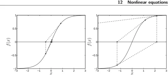
12 Nonlinear equations 167 12.1 Iterative algorithms . . . 167
12.2 Bisection method . . . 168
12.3 Newton’s method for one equation with one variable . . . 170
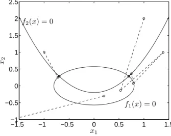
12.4 Newton’s method for sets of nonlinear equations . . . 172
12.5 Secant method . . . 173
12.6 Convergence analysis of Newton’s method . . . 175
Exercises . . . 180
13 Unconstrained minimization 185 13.1 Terminology . . . 185
13.2 Gradient and Hessian . . . 186
13.3 Optimality conditions . . . 189
13.4 Newton’s method for minimizing a convex function . . . 192
13.5 Newton’s method with backtracking . . . 194
13.6 Newton’s method for nonconvex functions . . . 200
Exercises . . . 202 14 Nonlinear least-squares 205 14.1 Definition . . . 205 14.2 Newton’s method . . . 206 14.3 Gauss-Newton method . . . 207 Exercises . . . 212
vi Contents 15 Linear optimization 219 15.1 Definition . . . 219 15.2 Examples . . . 220 15.3 Polyhedra . . . 223 15.4 Extreme points . . . 227 15.5 Simplex algorithm . . . 232 Exercises . . . 239
IV
Accuracy of numerical algorithms
241
16 Conditioning and stability 243 16.1 Problem conditioning . . . 243 16.2 Condition number . . . 244 16.3 Algorithm stability . . . 246 16.4 Cancellation . . . 246 Exercises . . . 249 17 Floating-point numbers 259 17.1 IEEE floating-point numbers . . . 25917.2 Machine precision . . . 260
17.3 Rounding . . . 261
Part I
Chapter 1
Vectors
1.1
Definitions and notation
Avectoris an ordered finite list of numbers. Vectors are usually written as vertical arrays, surrounded by brackets, as in
a= −1.1 0 3.6 −7.2 .
They can also be written as numbers separated by commas and surrounded by parentheses. In this notation style, the vector adefined above is written as
a= (−1.1,0,3.6,−7.2).
Theelements (orentries,coefficients,components) of a vector are the values in the array. The size (also called dimension or length) of the vector is the number of elements it contains. The vector aabove, for example, has size four. A vector of size nis called ann-vector. A 1-vector is considered to be the same as a number, i.e., we do not distinguish between the 1-vector [ 1.3 ] and the number 1.3.
Theith element of a vectorais denotedai, whereiis an integer index that runs from 1 to n, the size of the vector. For the example above,a3, the third element of the vectora, has the value 3.6.
The numbers or values of the elements in a vector are calledscalars. We will focus on the case that arises in most applications, where the scalars are real num-bers. In this case we refer to vectors as real vectors. The set of real n-vectors is denoted Rn. Occasionally other types of scalars arise. For example, the scalars can be complex numbers, in which case we refer to the vector as acomplex vector. The set of complex n-vectors is denotedCn. As another example, the scalars can be Boolean numbers.
4 1 Vectors Block vectors It is sometimes useful to define vectors by concatenating two or more vectors, as in a= bc d .
Ifbis anm-vector,c is ann-vector, anddisp-vector, this defines the (m+n+p )-vector
a= (b1, b2, . . . , bm, c1, c2, . . . , cn, d1, d2, . . . , dp).
Notational conventions Some authors try to use notation that helps the reader distinguish between vectors and scalars (numbers). For example, Greek letters (α, β, . . . ) might be used for numbers, and lower-case letters (a, x, f, . . . ) for vectors. Other notational conventions include vectors given in bold font (g), or vectors written with arrows above them (~a). These notational conventions are not standardized, so you should be prepared to figure out what things are (i.e., scalars or vectors) despite the author’s notational scheme (if any exists).
We should also give a couple of warnings concerning the subscripted index notationai. The first warning concerns the range of the index. In many computer languages, arrays are indexed fromi= 0 to n−1. But in standard mathematical notation, n-vectors are indexed fromi = 1 toi =n, so in this book, vectors will be indexed from i = 1 to i = n. The next warning concerns an ambiguity in the notation ai, used for the ith element of a vector a. The same notation will occasionally refer to the ith vector in a collection or list ofk vectors a1, . . . , ak. Whethera3means the third element of a vectora(in which casea3 is a number), or the third vector in some list of vectors (in which casea3is a vector) will be clear from the context.
1.2
Zero and unit vectors
A zero vector is a vector with all elements equal to zero. Sometimes the zero vector of sizenis written as 0n, where the subscript denotes the size. But usually a zero vector is denoted just 0, the same symbol used to denote the number 0. In this case you have to figure out the size of the zero vector from the context. (We will see how this is done later.)
Even though zero vectors of different sizes are different vectors, we use the same symbol 0 to denote them. In programming this is calledoverloading: the symbol 0 is overloaded because it can mean different things depending on the context (e.g., the equation it appears in).
A (standard)unit vector is a vector with all elements equal to zero, except one element which is equal to one. The ith unit vector (of size n) is the unit vector withith element one, and is denoted ei. The vectors
e1= 10 0 , e2= 01 0 , e3= 00 1
1.3 Vector addition 5
are the three unit vectors of size 3. The notation for unit vectors is an example of the ambiguity in notation noted at the end of section 1.1. Here,eidenotes theith unit vector, and not theith element of a vectore. As with zero vectors, the size of ei is usually determined from the context.
We use the notation1n for then-vector with all its elements equal to one. We also write 1if the size of the vector can be determined from the context. (Some authors useeto denote a vector of all ones, but we will not use this notation.)
1.3
Vector addition
Two vectorsof the same size can be added together by adding the corresponding elements, to form another vector of the same size. Vector addition is denoted by the symbol +. (Thus the symbol + is overloaded to mean scalar addition when scalars appear on its left- and right-hand sides, and vector addition when vectors appear on its left- and right-hand sides.) For example,
07 3 + 12 0 = 19 3 .
Vector subtraction is similar. As an example,
1 9 − 1 1 = 0 8 .
The following properties of vector addition are easily verified.
• Vector addition is commutative: ifaandb are vectors of the same size, then a+b=b+a.
• Vector addition is associative: (a+b) +c =a+ (b+c). We can therefore write both asa+b+c.
• a+ 0 = 0 +a=a. Adding the zero vector to a vector has no effect. (This is an example where the size of the zero vector follows from the context: it must be the same as the size ofa.)
Some languages for manipulating vectors define (overload) the sum of a vector and a scalar as the vector obtained by adding the scalar to each element of the vector. This is not standard mathematical notation, however, so we will not use it. In our (more standard) notation, we can express the vector obtained by adding the scalarγ to each element of the vectoraasa+γ1(using scalar multiplication, our next topic).
6 1 Vectors
1.4
Scalar-vector multiplication
Another operation isscalar multiplication orscalar-vector multiplication, in which a vector is multiplied by a scalar (i.e., number), which is done by multiplying every element of the vector by the scalar. Scalar multiplication is denoted by juxtaposition, with the scalar on the left, as in
(−2) 19 6 = −−182 −12 .
(Some people use scalar multiplication on the right, but this is nonstandard. An-other nonstandard notation you might see is a/2 instead of (1/2)a.) The scalar product (−1)a is written simply as −a. Note that 0a = 0 (where the left-hand zero is the scalar zero, and the right-hand zero is a vector zero of the same size asa).
Scalar multiplication obeys several laws that are easy to figure out from the definition. Ifais a vector andβ,γare scalars, then
(β+γ)a=βa+γa.
Scalar multiplication, like ordinary multiplication, has higher precedence than vec-tor addition, so the right-hand side here, βa+γa, means (βa) + (γa). It is useful to identify the symbols appearing in this formula above. The + symbol on the left is addition of scalars, while the + symbol on the right denotes vector addi-tion. Another simple property is (βγ)a =β(γa), where β and γ are scalars and a is a vector. On the left-hand side we see scalar-scalar multiplication (βγ) and scalar-vector multiplication; on the right we see two scalar-vector products.
Linear combinations Ifa1, . . . , am aren-vectors, andβ1, . . . , βm are scalars, the n-vector
β1a1+· · ·+βmam
is called a linear combination of the vectors a1, . . . , an. The scalars β1, . . . , βm are called the coefficients of the linear combination. As a simple but important application, we can write any vectoraas a linear combination of the standard unit vectors, as a=a1e1+· · ·+anen. (1.1) A specific example is −31 5 = (−1) 10 0 + 3 01 0 + 5 00 1 .
1.5 Inner product 7
1.5
Inner product
The (standard)inner product (also calleddot product) of twon-vectors is defined as the scalar
aTb=a1b1+a2b2+· · ·+anbn.
(The origin of the superscript in aT will be explained in chapter 2.) Some other notations for the inner product areha, bi,ha|bi, (a, b), anda·b. As you might guess, there is also a vector outer product, which we will encounter later, in chapter 2.
The inner product satisfies some simple properties that are easily verified from the definition. Ifa,b, andcare vectors of the same size, andγis a scalar, we have the following.
• aTb=bTa. The inner product is commutative: the order of the two vector arguments does not matter.
• (γa)Tb=γ(aTb), so we can write both asγaTb.
• (a+b)Tc =aTc+bTc. The inner product can be distributed across vector addition.
These can be combined to obtain other identities, such as aT(γb) = γ(aTb), or aT(b+γc) =aTb+γaTc.
Examples • eT
ia=ai. The inner product of a vector with the ith standard unit vector gives (or ‘picks out’) theith element a.
• 1Ta=a1+· · ·+an. The inner product of a vector with the vector of ones gives the sum of the elements of the vector.
• aTa=a2
1+· · ·+a2n. The inner product of a vector with itself gives the sum of the squares of the elements of the vector.
• Ifaand b aren-vectors, each of whose elements are either 0 or 1, thenaTb gives the total number of indices for whichai andbi are both one.
1.6
Linear functions
The notationf :Rn →Rmeans thatf is a function that maps realn-vectors to real numbers, i.e., it is a scalar valued function ofn-vectors. If xis an n-vector, thenf(x) denotes the value of the functionf atx, which is a scalar. We can also interpretf as a function ofnscalars, in which case we writef(x) as
8 1 Vectors
1.6.1
Inner products and linear functions
Supposea is ann-vector. We can define a scalar valued function f of n-vectors, given by
f(x) =aTx=a1x1+a2x2+· · ·+anxn (1.2) for any n-vector x. This function gives the inner product of its n-dimensional argument x with some (fixed) n-vector a. We can also think of f as forming a weighted sum of the elements ofx; the elements ofagive the weights.
Superposition and linearity The functionf defined in (1.2) satisfies the property f(αx+βy) = aT(αx+βy)
= aT(αx) +aT(βy) = α(aTx) +β(aTy) = αf(x) +βf(y)
for all n-vectors x, y, and all scalars α, β. This property is called superposition. A function that satisfies the superposition property is called linear. We have just showed that the inner product with a fixed vector is a linear function.
The superposition equality
f(αx+βy) =αf(x) +βf(y) (1.3) looks deceptively simple; it is easy to read it as just a re-arrangement of the paren-theses and the order of a few terms. But in fact it says a lot. On the left-hand side, the term αx+βy involves vector addition and scalar-vector multiplication. On the right-hand side,αf(x) +βf(y) involves ordinaryscalar multiplication and scalar addition.
Inner product representation of a linear function The converse is also true: If a function is linear, then it can be expressed as the inner product with some fixed vector. Supposef is a scalar valued function of n-vectors, and is linear,i.e.,
f(αx+βy) =αf(x) +βf(y)
for all n-vectorsx, y, and all scalarsα, β. Then there is ann-vector asuch that f(x) =aTxfor allx. We callaTxthe inner product representation off.
To see this, we use the identity (1.1) to express an arbitrary n-vector x as x=x1e1+· · ·+xnen. Iff is linear, then
f(x) = f(x1e1+x2e2+· · ·+xnen) = x1f(e1) +f(x2e2+· · ·+xnen) = x1f(e1) +x2f(e2) +f(x3e3+· · ·+xnen) .. . = x1f(e1) +x2f(e2) +· · ·+xnf(en) = aTx
1.6 Linear functions 9
witha= (f(e1), f(e2), . . . , f(en)). The formula just derived,
f(x) =x1f(e1) +x2f(e2) +· · ·+xnf(en) (1.4) which holds for any linear scalar valued function f, has several interesting impli-cations. Suppose, for example, that the linear function f is given as a subroutine (or a physical system) that computes (or results in the output)f(x) when we give the argument (or input)x. Once we have foundf(e1), . . . , f(en), byncalls to the subroutine (ornexperiments), we can predict (or simulate) whatf(x) will be, for any vectorx, using the formula (1.4).
The representation of a linear function f as f(x) = aTx is unique. In other words, there is only one vectorafor whichf(x) =aTxholds for allx. To see this, suppose that we havef(x) =aTxfor allx, and alsof(x) =bTxfor allx. Taking x = ei, we have f(ei) = aTei = ai, using the formula f(x) = aTx. Using the formula f(x) =bTx, we havef(ei) =bTei =bi. These two numbers must be the same, so we have ai =bi. Repeating this argument for i = 1, . . . , n, we conclude that the corresponding elements inaandbare the same, soa=b.
Examples
• Average. The average of the elements ofx,f(x) = (x1+x2+· · ·+xn)/n, is a linear function. It can be expressed asf(x) =aTxwith
a= (1 n, 1 n, . . . , 1 n) = 1 n1.
• Maximum. The maximum element of x, f(x) = maxkxk, is not a linear function. We can show this is by a counterexample. Choose n = 2, x = (1,−1), y= (−1,1),α= 1, β= 1. Then
f(αx+βy) = 06=αf(x) +βf(y) = 2.
Affine functions A linear function plus a constant is called anaffine function. A functionf :Rn →Ris affine if and only if it can be expressed asf(x) =aTx+b for some n-vector aand scalar b. For example, the function on 3-vectors defined by
f(x) = 2.3−2x1+ 1.3x2−x3, is affine, withb= 2.3,a= (−2,1.3,−1).
Any affine scalar valued function satisfies the following variation on the super-position property:
f(αx+βy) =αf(x) +βf(y),
for alln-vectorsx,y, and all scalarsα,β that satisfyα+β= 1. (In the definition of linearity, there is no requirement that the coefficients α and β sum to one.) The converse is also true: Any scalar valued function that satisfies this property is affine. An analog of the formula (1.4) for linear functions is
10 1 Vectors
which holds whenfis affine, andxis anyn-vector (see exercise 1.19). This formula shows that for an affine function, once we know then+ 1 numbersf(0),f(e1), . . . , f(en), we can predict (or reconstruct or evaluate)f(x) for anyn-vectorx.
In some contexts affine functions are called linear. For example, y = αx+β is sometimes referred to as a linear function of x. As another common example, the first-order Taylor approximation off (described below) is in general an affine function, but is often called linear. In this book, however, we will distinguish between linear and affine functions.
1.6.2
Linearization of a scalar valued function
Supposef :Rn→Ris continuously differentiable,i.e., the partial derivatives ∂f(ˆx)
∂xk = limt→0
f(ˆx+tek)−f(ˆx)
t , k= 1, . . . , n,
exist at all ˆx, and are continuous functions of ˆx. Thegradient off, at a vector ˆx, is the vector of first partial derivatives evaluated at ˆx, and is denoted∇f(ˆx):
∇f(ˆx) = ∂f(ˆx)/∂x1 ∂f(ˆx)/∂x2 .. . ∂f(ˆx)/∂xn .
The first-order Taylor approximation of f around (or near) ˆx is defined as the functionfaff defined by
faff(x) = f(ˆx) + n X k=1 ∂f(ˆx) ∂xk (xk−xkˆ ) = f(ˆx) +∇f(ˆx)T(x−xˆ). (1.5) The functionfaff is also called the linearization off at (or near) the point ˆx, and gives a very good approximation of f(x) for x near ˆx. If n = 1, the gradient is simply the first derivativef′(ˆx), and the first-order approximation reduces to
faff(x) =f(ˆx) +f′(ˆx)(x−xˆ).
The first-order Taylor approximationfaff is an affine function ofx; we can write it asfaff(x) =aTx+b, where
a=∇f(ˆx), b=f(ˆx)− ∇f(ˆx)Txˆ (but the formula given in (1.5) is probably easier to understand).
The first-order approximation is often expressed in the following way. Define y = f(x) and ˆy = f(ˆx). We define δy and δx (which are to be interpreted as indivisible two-character symbols, not the products ofδandy orx) as
1.7 Euclidean norm 11
These are called theyandxdeviations (from ˆyand ˆx) respectively. The first-order approximation can be expressed as
δy≈ ∇f(ˆx)Tδx,
for xnear ˆx. Thus, the y deviation is approximately a linear function of the x deviation.
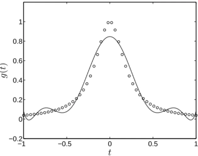
Example We will find the first-order Taylor approximation of the function f : R2→R, defined by
f(x) =ex1+x2−1+ex1−x2−1+e−x1−1, (1.6) at the point ˆx= 0. Its gradient, at a general point ˆx, is
∇f(ˆx) = " exˆ1+ˆx2−1+exˆ1−xˆ2−1−e−xˆ1−1 exˆ1+ˆx2−1−eˆx1−ˆx2−1 # , (1.7)
so ∇f(0) = (1/e,0). The first-order approximation of f around ˆx= 0 is faff(x) = f(0) +∇f(0)T(x−0)
= 3/e+ (1/e,0)Tx = 3/e+x1/e.
For x1 and x2 near zero, the function (x1+ 3)/e therefore gives a very good ap-proximation off(x).
1.7
Euclidean norm
The Euclidean norm of a vector x, denoted kxk, is the square root of the sum of the squares if its elements,
kxk=
q
x2
1+x22+· · ·+x2n.
The Euclidean norm is sometimes written with a subscript 2, as kxk2. We can express the Euclidean norm in terms of the inner product ofxwith itself:
kxk=√xTx.
When x is a scalar, i.e., a 1-vector, the Euclidean norm is the same as the absolute value ofx. Indeed, the Euclidean norm can be considered a generalization or extension of the absolute value or magnitude, that applies to vectors. The double bar notation is meant to suggest this.
Some important properties of norms are given below. Herexandy are vectors, andβ is a scalar.
12 1 Vectors • Homogeneity. kβxk=|β|kxk.
• Triangle inequality. kx+yk ≤ kxk+kyk.
• Nonnegativity. kxk ≥0.
• Definiteness. kxk= 0 only ifx= 0.
The last two properties together, which state that the norm is always nonnegative, and zero only when the vector is zero, are called positive definiteness. The first, third, and fourth properties are easy to show directly from the definition of the norm. Establishing the second property, the triangle inequality, is not as easy; we will give a derivation a bit later.
Root-mean-square value The Euclidean norm is related to theroot-mean-square (RMS) value of a vectora, defined as
RMS(x) = r 1 n(x 2 1+· · ·+x2n) = 1 √ nkxk.
Roughly speaking, the RMS value of a vector x tells us what a ‘typical’ value of
|xi|is, and is useful when comparing norms of vectors of different sizes.
Euclidean distance We can use the norm to define theEuclidean distancebetween two vectorsaandbas the norm of their difference:
dist(a, b) =ka−bk.
For dimensions one, two, and three, this distance is exactly the usual distance between points with coordinates a and b. But the Euclidean distance is defined for vectors of any dimension; we can refer to the distance between two vectors of dimension 100.
We can now explain where the triangle inequality gets its name. Consider a triangle in dimension two or three, whose vertices have coordinates a, b, and c. The lengths of the sides are the distances between the vertices,
ka−bk, kb−ck, ka−ck.
The length of any side of a triangle cannot exceed the sum of the lengths of the other two sides. For example, we have
ka−ck ≤ ka−bk+kb−ck. (1.8) This follows from the triangle inequality, since
1.8 Angle between vectors 13 General norms Any real valued functionf that satisfies the four properties above
(homogeneity, triangle inequality, nonnegativity, and definiteness) is called avector norm, and is usually written asf(x) =kxkmn, where the subscript is some kind of identifier or mnemonic to identify it.
Two common vector norms are the 1-normkak1 and the∞-normkak∞, which
are defined as
kak1=|a1|+|a2|+· · ·+|an|, kak∞= max
k=1,...,n|ak|.
These norms measure the sum and the maximum of the absolute values of the elements in a vector, respectively. The 1-norm and the ∞-norm arise in some recent and advanced applications, but we will not encounter them much in this book. When we refer to the norm of a vector, we always mean the Euclidean norm.
Weighted norm Another important example of a general norm is a weighted norm, defined as
kxkw=
p
(x1/w1)2+· · ·+ (xn/wn)2,
wherew1, . . . , wnare given positiveweights, used to assign more or less importance to the different elements of then-vectorx. If all the weights are one, the weighted norm reduces to the (‘unweighted’) Euclidean norm.
Weighted norms arise naturally when the elements of the vectorxhave different physical units, or natural ranges of values. One common rule of thumb is to choose wi equal to the typical value of |xi| in the application or setting. These weights bring all the terms in the sum to the same order, one. We can also imagine that the weights contain the same physical units as the elements xi, which makes the terms in the sum (and therefore the norm as well) unitless.
For example, consider an application in whichx1represents a physical distance, measured in meters, and has typical values on the order of±105m, andx2represents a physical velocity, measured in meters/sec, and has typical values on the order of 10m/s. In this case we might wish to use the weighted norm
kxkw=
p
(x1/w1)2+ (x2/w2)2,
with w1 = 105 and w2 = 10, to measure the size of a vector. If we assign to w1 physical units of meters, and to w2 physical units of meters per second, the weighted norm kxkw becomes unitless.
1.8
Angle between vectors
Cauchy-Schwarz inequality An important inequality that relates Euclidean norms and inner products is theCauchy-Schwarz inequality:
|aTb| ≤ kak kbk
for allaandb. This can be shown as follows. The inequality clearly holds ifa= 0 orb= 0 (in this case, both sides of the inequality are zero). Supposea6= 0,b6= 0,
14 1 Vectors
and consider the function f(t) =ka+tbk2, wheretis a scalar. We havef(t)≥0 for allt, since f(t) is a sum of squares. By expanding the square of the norm we can writef as
f(t) = (a+tb)T(a+tb)
= aTa+tbTa+taTb+t2bTb = kak2+ 2taTb+t2kbk2.
This is a quadratic function with a positive coefficient oft2. It reaches its minimum where f′(t) = 2aTb+ 2tkbk2 = 0, i.e., at ¯t = −aTb/kbk2. The value off at the minimum is
f(¯t) =kak2−(a
Tb)2
kbk2 .
This must be nonnegative since f(t) ≥0 for allt. Therefore (aTb)2 ≤ kak2kbk2. Taking the square root on each side gives the Cauchy-Schwarz inequality.
This argument also reveals the conditions onaandb under which they satisfy the Cauchy-Schwarz inequality with equality. Supposea and b are nonzero, with
|aTb|=kak kbk. Then
f(¯t) =ka+ ¯tbk2=kak2−(aTb)2/kbk2= 0,
and soa+ ¯tb= 0. Thus, if the Cauchy-Schwarz inequality holds with equality for nonzeroa and b, then aand b are scalar multiples of each other. If ¯t < 0,a is a positive multiple ofb(and we say the vectors arealigned). In this case we have
aTb=−tb¯Tb=|¯t|kbk2=k−¯tbk kbk=kak kbk.
If ¯t >0,ais a negative multiple ofb(and we say the vectors areanti-aligned). We have
aTb=−tb¯Tb=−|¯t|kbk2=−k−¯tbkkbk=−kakkbk.
Verification of triangle inequality We can use the Cauchy-Schwarz inequality to verify the triangle inequality. Letaandbbe any vectors. Then
ka+bk2 = kak2+ 2aTb+kbk2 ≤ kak2+ 2kakkbk+kbk2
= (kak+kbk)2,
where we used the Cauchy-Schwarz inequality in the second line. Taking the square root we get the triangle inequality,ka+bk ≤ kak+kbk.
Correlation coefficient Supposeaandbare nonzero vectors of the same size. We define theircorrelation coefficient as
ρ= a
Tb
kak kbk.
This is a symmetric function of the vectors: the correlation between a and b is the same as the correlation coefficient between b and a. The Cauchy-Schwarz
1.8 Angle between vectors 15
inequality tells us that the correlation coefficient ranges between −1 and +1. For this reason, the correlation coefficient is sometimes expressed as a percentage. For example, ρ= 30% meansρ= 0.3, i.e., aTb= 0.3kakkbk. Very roughly speaking, the correlation coefficientρtells us how well the shape of one vector (say, if it were plotted versus index) matches the shape of the other. We have already seen, for example, that ρ = 1 only if the vectors are aligned, which means that each is a positive multiple of the other, and thatρ=−1 occurs only when each vector is a negative multiple of the other.
Two vectors are said to be highly correlated if their correlation coefficient is near one, anduncorrelated if the correlation coefficient is small.
Example Conisider x= 0.1 −0.3 1.3 −0.3 −3.3 y= 0.2 −0.4 3.2 −0.8 −5.2 z= 1.8 −1.0 −0.6 1.4 −0.2 . We have kxk= 3.57, kyk= 6.17, kzk= 2.57, xTy= 21.70, xTz=−0.06, and therefore ρxy= x Ty kxk kyk = 0.98, ρxz = xTz kxk kzk =−0.007.
We see that x and y are highly correlated (y is roughly equal to x scaled by 2). The vectors xandz on the other hand are almost uncorrelated.
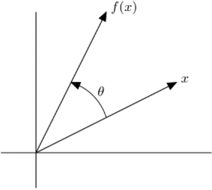
Angle between vectors Theangle between two nonzero vectors a, bwith corre-lation coefficientρis defined as
θ= arccosρ= arccos
aTb
kak kbk
where arccos denotes the inverse cosine, normalized to lie in the interval [0, π]. In other words, we define θas the unique number in [0, π] that satisfies
aTb=kak kbkcosθ.
The angle betweenaandbis sometimes written as6 (a, b). The angle is a symmetric
function of a and b: we have 6 (a, b) = 6 (b, a). The angle between vectors is
sometimes expressed in degrees. For example, 6 (a, b) = 30◦ means 6 (a, b) =π/6,
i.e.,aTb= (1/2)kakkbk.
The angle coincides with the usual notion of angle between vectors, when they have dimension two or three. But the definition of angle is more general; we can refer to the angle between two vectors with dimension 100.
16 1 Vectors Acute and obtuse angles Angles are classified according to the sign ofaTb.
• If the angle isπ/2 = 90◦,i.e.,aTb= 0, the vectors are said to beorthogonal. This is the same as the vectors being uncorrelated. We writea⊥b ifaand b are orthogonal.
• If the angle is zero, which meansaTb=kakkbk, the vectors arealigned. This is the same as saying the vectors have correlation coefficient 1, or that each vector is a positive multiple of the other (assuming the vectors are nonzero).
• If the angle is π= 180◦, which meansaTb=−kak kbk, the vectors are anti-aligned. This means the correlation coefficient is −1, and each vector is a negative multiple of the other (assuming the vectors are nonzero).
• If 6 (a, b) ≤π/2 = 90◦, the vectors are said to make an acute angle. This
is the same as saying the vectors have nonnegative correlation coefficient, or nonnegative inner product, aTb≥0.
• If 6 (a, b) ≥π/2 = 90◦, the vectors are said to make anobtuse angle. This
is the same as saying the vectors have nonpositive correlation coefficient, or nonpositive inner product,aTb≤0.
Orthonormal set of vectors A vectorais said thenormalized, or aunit vector, if
kak= 1. A set of vectors{a1, . . . , ak}isorthogonalifai⊥ajfor anyi,jwithi6=j, i, j= 1, . . . , k. It is important to understand that orthogonality is an attribute of a set of vectors, and not an attribute of vectors individually. It makes no sense to say that a vectora is orthogonal; but we can say that{a} (the set whose only element isa) is orthogonal. But this last statement is true for any nonzero a, and so is not informative.
A set of normalized and orthogonal vectors is also called orthonormal. For example, the set of 3-vectors
00 −1 , √1 2 11 0 , √1 2 −11 0 , is orthonormal.
Orthonormal sets of vectors have many applications. Suppose a vector x is a linear combination of a1, . . . , ak, where {a1, . . . , ak} is an orthonormal set of vectors,
x=β1a1+· · ·+βkak.
Taking the inner product of the left and right-hand sides of this equation withai yields
aTi x = aTi(β1a1+· · ·+βkak) = β1aTia1+· · ·+βkaTiak = βi,
sinceaT
iaj = 1 for i=j, andaTiaj = 0 for i6=j. So if a vector can be expressed as a linear combination of an orthonormal set of vectors, we can easily find the coefficients of the linear combination by taking the inner products with the vectors.
1.9 Vector inequality 17
1.9
Vector inequality
In some applications it is useful to define inequality between vectors. If xand y are vectors of the same size, say n, we define x ≤y to mean that x1 ≤y1, . . . , xn≤yn,i.e., each element ofxis less than or equal to the corresponding element ofy. We definex≥y in the obvious way, to meanx1≥y1, . . . ,xn≥yn. We refer to x≤y orx≥yas (nonstrict) vector inequalities.
We define strict inequalities in a similar way: x < y means x1 < y1, . . . , xn < yn, and x > y means x1 > y1, . . . , xn > yn. these are called strict vector inequalities.
18 1 Vectors
Exercises
Block vectors
1.1 Some block vector operations. Letxbe a block vector with two vector elements,
x= a b ,
whereaandbare vectors of sizenandm, respectively. (a) Show that
γx= γa γb , whereγis a scalar. (b) Show that kxk= kak2+kbk21/2= kak kbk . (Note that the norm on the right-hand side is of a 2-vector.) (c) Letybe another block vector
y= c d ,
wherecanddare vectors of sizenandm, respectively. Show that
x+y= a+c b+d , xTy=aTc+bTd. Linear functions
1.2 Which of the following scalar valued functions on Rn are linear? Which are affine? If a function is linear, give its inner product representation, i.e., an n-vector a such that
f(x) =aTxfor allx. If it is affine, giveaandbsuch thatf(x) =aTx+bholds for allx. If it is neither, give specificx,y,α, andβfor which superposition fails,i.e.,
f(αx+βy)6=αf(x) +βf(y).
(Providedα+β= 1, this shows the function is neither linear nor affine.) (a) The spread of values of the vector, defined asf(x) = maxkxk−minkxk.
(b) The difference of the last element and the first,f(x) =xn−x1.
(c) The difference of the squared distances to two fixed vectorscandd, defined as
f(x) =kx−ck2− kx−dk2.
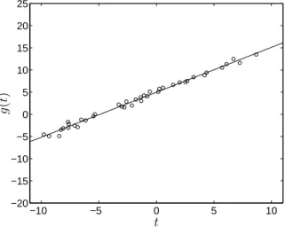
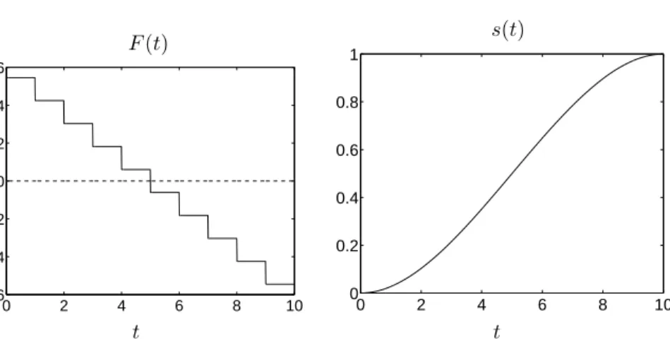
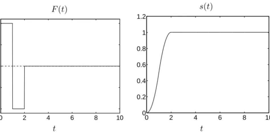
1.3 A unit mass moves on a straight line (in one dimension). The position of the mass at timetis denoted bys(t), and its derivatives (the velocity and acceleration) bys′(t) and
s′′(t). The position as a function of time can be determined from Newton’s second law
s′′(t) =F(t),
whereF(t) is the force applied at timet, and the initial conditionss(0),s′(0). We assume
F(t) is piecewise-constant, and is kept constant in intervals of one second. The sequence of forcesF(t), for 0≤t <10s, can then be represented by a 10-vectorx, with
Exercises 19
(a) Suppose the initial position and velocity are zero (s(0) =s′(0) = 0). Derive expres-sions for the velocitys′(10) and positions(10) at timet= 10. Show thats(10) and
s′(10) are linear functions ofx.
(b) How does the answer change if we start from nonzero initial position or velocity?
1.4 Deviation of middle element value from average. Supposexis an-vector, withn= 2m−1 andm≥1. We define the middle element value ofxasxm. Define
f(x) =xm− 1 n n X i=1 xi,
which is the difference between the middle element value and the average of the coefficients inx. Expressfin the formf(x) =aTx, whereais ann-vector.
1.5 The temperatureT of an electronic device containing three processors is an affine func-tion of the power dissipated by the three processors, P = (P1, P2, P3). When all three processors are idling, we have P = (10,10,10), which results in a temperatureT = 30. When the first processor operates at full power and the other two are idling, we have
P = (100,10,10), and the temperature rises toT = 60. When the second processor op-erates at full power and the other two are idling, we have P = (10,100,10) andT = 70. When the third processor operates at full power and the other two are idling, we have
P = (10,10,100) andT = 65. Now suppose that all three processors are operated at the same powerP. How large canP be, if we require thatT ≤85?
1.6 Taylor approximation of norm. Find an affine approximation of the functionf(x) =kxk, near a given nonzero vector ˆx. Check your approximation formula as follows. First, choose ˆxas a random 5-vector. (In MATLAB, for example, you can use the command hatx = randn(5,1).) Then choose several vectorsxrandomly, withkx−xˆkon the order of 0.1kxˆk (in MATLAB, usingx = hatx + 0.1*randn(5,1)), and comparef(x) =kxk
andf(ˆx) =kxˆk. Norms and angles
1.7 Verify that the following identities hold for any two vectorsaandbof the same size. (a) (a+b)T(a−b) =kak2− kbk2.
(b) ka+bk2+ka−bk2= 2(kak2+kbk2).
1.8 When does the triangle inequality hold with equality, i.e., what are the conditions ona
andbto haveka+bk=kak+kbk?
1.9 Show thatka+bk ≥kak − kbk.
1.10 Approximating one vector with a scalar multiple of another. Suppose we have a nonzero vectorxand a vectoryof the same size.
(a) How do you choose the scalartso thatktx−ykis minimized? SinceL={tx|t∈R}
describes the line passing through the origin and the pointx, the problem is to find the point inLclosest to the pointy. Hint. Work withktx−yk2.
(b) Lett⋆be the value found in part (a), and letz=t⋆x. Show that (y−z)⊥x.
(c) Draw a picture illustrating this exercise, for 2-vectors. Show the pointsxandy, the lineL, the pointz, and the line segment betweenyandz.
(d) Expressd=kz−yk, which is the closest distance of a point on the lineL and the pointy, in terms ofkykandθ=6 (x, y).
1.11 Minimum distance between two lines. Find the minimum distance between the lines
L={u+tv|t∈R}, L˜={u˜+ ˜t˜v|t˜∈R}.
20 1 Vectors
1.12 H¨older inequality. The Cauchy-Schwarz inequality states that|xTy| ≤ kxkkyk, for any vectorsxandy. The H¨older inequality gives another bound on the absolute value of the inner product, in terms of the product of norms: |xTy| ≤ kxk∞kyk1. (These are the∞ and 1-norms, defined on page 13.) Derive the H¨older inequality.
1.13 Norm of linear combination of orthonormal vectors. Suppose{a1, . . . , ak}is an
orthonor-mal set ofn-vectors, andx=β1a1+· · ·+βkak. Expresskxkin terms ofβ1, . . . ,βk. 1.14 Relative deviation between vectors. Supposeaandbare nonzero vectors of the same size.
The relative deviation ofbfromais defined as the distance betweenaandb, divided by the norm ofa,
ηab=ka−bk kak .
This is often expressed as a percentage. The relative deviation is not a symmetric function ofaandb; in general, ηab6=ηba.
Suppose ηab = 0.1 (i.e., 10%). How big and how small can be ηba be? Explain your
reasoning.
1.15 Average and norm. Use the Cauchy-Schwarz inequality to prove that
−√1 nkxk ≤ 1 n n X i=1 xi≤ 1 √ nkxk
for alln-vectorsx. In other words, the average of the elements of a vector lies between
±1/√n times its norm. What are the conditions on x to have equality in the upper bound? When do we have equality in the lower bound?
1.16 Use the Cauchy-Schwarz inequality to prove that 1 n n X k=1 xk≥ 1 n n X k=1 1 xk !−1
for alln-vectorsxwith positive elementsxk.
The left-hand side of the inequality is the arithmetic mean (average) of the numbersxk;
the right-hand side is called the harmonic mean.
1.17 Euclidean norm of sum. Derive a formula forka+bkin terms ofkak,kbk, andθ=6 (a, b). Use this formula to show the following:
(a) a⊥bif and only ifka+bk=pkak2+kbk2.
(b) aandbmake an acute angle if and only ifka+bk ≥pkak2+kbk2. (c) aandbmake an obtuse angle if and only ifka+bk ≤pkak2+kbk2. Draw a picture illustrating each case (inR2).
1.18 Angle between nonnegative vectors. Show that the angle between two nonnegative vectors
xandylies between 0 andπ/2. When are two nonnegative vectorsxandyorthogonal?
1.19 Letf:Rn→Rbe an affine function. Show thatf can be expressed asf(x) =aTx+b
for somea∈Rnandb∈R.
1.20 Decoding using inner products. An input signal is sent over a noisy communication chan-nel. The channel adds a small noise to the input signal, and attenuates it by an unknown factorα. We represent the input signal as ann-vectoru, the output signal as ann-vector
v, and the noise signal as ann-vector w. The elementsuk,vk,wk give the values of the
signals at timek. The relation betweenuandvis
v=αu+w.
Exercises 21 0 50 100 150 200 −1 0 1 k uk 0 50 100 150 200 −1 0 1 k vk
Now suppose we know that the input signal u was chosen from a set of four possible signals
x(1), x(2), x(3), x(4)∈Rn.
We know these signalsx(i), but we do not know which one was used as input signal u. Our task is to find a simple, automated way to estimate the input signal, based on the received signal v. There are many ways to do this. One possibility is to calculate the angleθkbetweenvandx(k), via the formula
cosθk= v Tx(k)
kvk kx(k)k and pick the signalx(k)that makes the smallest angle withv.
Download the file ch1ex20.mfrom the class webpage, save it in your working directory, and execute it in MATLAB using the command[x1,x2,x3,x4,v] = ch1ex20. The first four output arguments are the possible input signalsx(k),k= 1,2,3,4. The fifth output argument is the received (output) signalv. The length of the signals isn= 200.
(a) Plot the vectorsv,x(1),x(2),x(3),x(4). Visually, it should be obvious which input signal was used to generatev.
(b) Calculate the angles of v with each of the four signals x(k). This can be done in MATLAB using the command
acos((v’*x)/(norm(x)*norm(v)))
(which returns the angle betweenxandvin radians). Which signalx(k)makes the smallest angle withv? Does this confirm your conclusion in part (a)?
1.21 Multiaccess communication. A communication channel is shared by several users (trans-mitters), who use it to send binary sequences (sequences with values +1 and −1) to a receiver. The following technique allows the receiver to separate the sequences transmitted by each transmitter. We explain the idea for the case with two transmitters.
We assign to each transmitter a different signal or code. The codes are represented as
n-vectorsuandv: uis the code for user 1,vis the code for user 2. The codes are chosen to be orthogonal (uTv= 0). The figure shows a simple example of two orthogonal codes of lengthn= 100. 0 20 40 60 80 100 0 0.2 0.4 0.6 0.8 1 k uk 0 20 40 60 80 100 −1 −0.5 0 0.5 1 k vk
22 1 Vectors
Suppose user 1 wants to transmit a binary sequence b1,b2, . . . ,bm (with valuesbi = 1
orbi=−1), and user 2 wants to transmit a sequencec1,c2, . . . ,cm(with valuesci= 1
orci=−1). From these sequences and the user codes, we construct two signalsxandy,
both of lengthmn, as follows:
x= b1u b2u .. . bmu , y= c1v c2v .. . cmv .
(Note that here we use block vector notation: xandyconsist ofmblocks, each of sizen. The first block ofxisb1u, the code vector umultiplied with the scalarb1, etc.) User 1 sends the signalxover the channel, and user 2 sends the signaly. The receiver receives the sum of the two signals. We write the received signal asz:
z=x+y= b1u b2u .. . bmu + c1v c2v .. . cmv .
The figure shows an example where we use the two code vectors uandv shown before. In this examplem= 5, and the two transmitted sequences areb= (1,−1,1,−1,−1) and
c= (−1,−1,1,1,−1). 0 100 200 300 400 500 −1 0 1 0 100 200 300 400 500 −1 0 1 0 100 200 300 400 500 −2 0 2 k xk yk zk
How can the receiver recover the two sequences bk and ck from the received signal z?
Let us denote the first block (consisting of the firstn values) of the received signalz as
z(1): z(1)=b1u+c1v. If we make the inner product ofz(1)withu, and use the fact that
uTv= 0, we get
uTz(1)=uT(b1u+c1v) =b1uTu+c1uTv=b1kuk2. Similarly, the inner product withvgives
Exercises 23
We see thatb1 andc1 can be computed from the received signal as
b1=u
Tz(1)
kuk2 , c1 =
vTz(1)
kvk2 .
Repeating this for the other blocks ofz allows us to recover the rest of the sequences b
andc: bk= u Tz(k) kuk2 , ck= vTz(k) kvk2 , ifz(k) is thekth block ofz.
Download the filech1ex21.mfrom the class webpage, and run it in MATLAB as[u,v,z] = ch1ex21. This generates two code vectors uand v of length n = 100, and a received signalz of
lengthmn= 500. (The code vectorsuandvare different from those used in the figures above.) In addition we added a small noise vector to the received signalz,i.e., we have
z= b1u b2u .. . bmu + c1v c2v .. . cmv +w wherewis unknown but small compared touandv.
(a) Calculate the angle between the code vectorsuand v. Verify that they are nearly (but not quite) orthogonal. As a result, and because of the presence of noise, the formulas forbk andck are not correct anymore. How does this affect the decoding
scheme? Is it still possible to compute the binary sequencesbandcfromz? (b) Compute (b1, b2, b3, b4, b5) and (c1, c2, c3, c4, c5).
Chapter 2
Matrices
2.1
Definitions and notation
Amatrix is a rectangular array of numbers written between brackets, as in
A= 10.3 14 −−20..31 00.1 4.1 −1 0 1.7 .
An important attribute of a matrix is its size or dimensions, i.e., the numbers of rows and columns. The matrix A above has 3 rows and 4 columns, so its size is 3×4. A matrix of sizem×nis called anm×n-matrix.
Theelements (orentries orcoefficients) of a matrix are the values in the array. The i, j element is the value in the ith row and jth column, denoted by double subscripts: the i, j element of a matrix A is denoted Aij or aij. The positive integers i and j are called the (row and column, respectively)indices. If A is an m×n-matrix, then the row indexiruns from 1 tomand the column indexj runs from 1 to n. For the example above,a13=−2.3,a32 =−1. The row index of the bottom left element (which has value 4.1) is 3; its column index is 1.
Ann-vector can be interpreted as ann×1-matrix; we do not distinguish between vectors and matrices with one column. A matrix with only one row,i.e., with size 1×n, is sometimes called arow vector. As an example,
w= −2.1 −3 0
is a row vector (or 1×3-matrix). A 1×1-matrix is considered to be the same as a scalar.
Asquare matrix has an equal number of rows and columns. A square matrix of sizen×n is said to be oforder n. A tall matrix has more rows than columns (sizem×nwithm > n). Awide matrix has more columns than rows (sizem×n withn > m).
All matrices in this course are real, i.e., have real elements. The set of real m×n-matrices is denotedRm×n.
26 2 Matrices Block matrices and submatrices In some applications it is useful to form matrices whose elements are themselves matrices, as in
A= B C D , E= E11 E12 E21 E22 ,
where B, C, D, E11, E12, E21, E22 are matrices. Such matrices are called block matrices; the elementsB,C, and Dare called blocks or submatrices. The subma-trices are sometimes named by indices, as in the second matrix E. Thus, E11 is the 1,1 block ofE.
Of course the block matrices must have the right dimensions to be able to fit together. Matrices in the same (block) row must have the same number of rows (i.e., the same ‘height’); matrices in the same (block) column must have the same number of columns (i.e., the same ‘width’). In the examples above, B,C, andD must have the same number of rows (e.g., they could be 2×3, 2×2, and 2×1). In the second example,E11 must have the same number of rows as E12, andE21 must have the same number of rows as E22. E11 must have the same number of columns asE21, andE12 must have the same number of columns asE22.
As an example, if C= 0 2 3 5 4 7 , D= 2 2 1 3 , then C D = 0 2 3 2 2 5 4 7 1 3 .
Using block matrix notation we can write an m×n-matrixAas A= B1 B2 · · · Bn ,
if we defineBk to be them×1-matrix (orm-vector)
Bk = a1k a2k .. . amk .
Thus, an m×n-matrix can be viewed as an ordered set of n vectors of size m. Similarly,A can be written as a block matrix with one block column andmrows:
A= C1 C2 .. . Cm ,
if we defineCk to be the 1×n-matrix
Ck= ak1 ak2 · · · akn .
In this notation, the matrix A is interpreted as an ordered collection of m row vectors of sizen.
2.2 Zero and identity matrices 27
2.2
Zero and identity matrices
A zero matrix is a matrix with all elements equal to zero. The zero matrix of size m×nis sometimes written as 0m×n, but usually a zero matrix is denoted just 0, the same symbol used to denote the number 0 or zero vectors. In this case the size of the zero matrix must be determined from the context.
An identity matrix is another common matrix. It is always square. Itsdiagonal elements, i.e., those with equal row and column index, are all equal to one, and its off-diagonal elements (those with unequal row and column indices) are zero. Identity matrices are denoted by the letterI. Formally, the identity matrix of size nis defined by
Iij =
1 i=j 0 i6=j. Perhaps more illuminating are the examples
1 0 0 1 , 1 0 0 0 0 1 0 0 0 0 1 0 0 0 0 1
which are the 2×2 and 4×4 identity matrices.
The column vectors of then×nidentity matrix are the unit vectors of sizen. Using block matrix notation, we can write
I= e1 e2 · · · en where ek is thekth unit vector of sizen(see section 1.2).
Sometimes a subscript denotes the size of a identity matrix, as inI4 or I2×2. But more often the size is omitted and follows from the context. For example, if
A= 1 2 3 4 5 6 , then I A 0 I = 1 0 1 2 3 0 1 4 5 6 0 0 1 0 0 0 0 0 1 0 0 0 0 0 1 .
The dimensions of the two identity matrices follow from the size ofA. The identity matrix in the 1,1 position must be 2×2, and the identity matrix in the 2,2 position must be 3×3. This also determines the size of the zero matrix in the 2,1 position.
The importance of the identity matrix will become clear in section 2.6.
2.3
Matrix transpose
IfAis anm×n-matrix, itstranspose, denotedAT (or sometimesA′), is then×m
-matrix given by (AT)
28 2 Matrices inAT. For example, 0 47 0 3 1 T = 0 7 3 4 0 1 .
If we transpose a matrix twice, we get back the original matrix: (AT)T =A. Note that transposition converts row vectors into column vectors and vice versa.
A square matrixAissymmetric ifA=AT,i.e.,aij =aji for alli, j.
2.4
Matrix addition
Two matrices of the same size can be added together. The result is another matrix of the same size, obtained by adding the corresponding elements of the two matrices. For example, 07 40 3 1 + 1 22 3 0 4 = 1 69 3 3 5 . Matrix subtraction is similar. As an example,
1 6 9 3 −I= 0 6 9 2 .
(This gives another example where we have to figure out the size of the identity matrix. Since you can only add or subtract matrices of the same size,Irefers to a 2×2 identity matrix.)
The following important properties of matrix addition can be verified directly from the definition.
• Matrix addition is commutative: if A andB are matrices of the same size, thenA+B=B+A.
• Matrix addition is associative: (A+B) +C =A+ (B+C). We therefore write both asA+B+C.
• A+ 0 = 0 +A=A. Adding the zero matrix to a matrix has no effect.
• (A+B)T =AT +BT. The transpose of a sum of two matrices is the sum of their transposes.
2.5
Scalar-matrix multiplication
Scalar multiplication of matrices is defined as for vectors, and is done by multiplying every element of the matrix by the scalar. For example
(−2) 1 69 3 6 0 = −−182 −−126 −12 0 .
2.6 Matrix-matrix multiplication 29
Note that 0A= 0 (where the left-hand zero is the scalar zero).
Several useful properties of scalar multiplication follow directly from the defini-tion. For example, (βA)T =β(AT) for a scalarβ and a matrixA. IfAis a matrix andβ,γare scalars, then
(β+γ)A=βA+γA, (βγ)A=β(γA).
2.6
Matrix-matrix multiplication
It is possible to multiply two matrices usingmatrix multiplication. You can multiply two matrices AandB provided their dimensions arecompatible, which means the number of columns of A equals the number of rows of B. SupposeA and B are compatible,e.g.,Ahas sizem×pandB has sizep×n. Then the product matrix C=ABis them×n-matrix with elements
cij = p
X
k=1
aikbkj=ai1b1j+· · ·+aipbpj, i= 1, . . . , m, j= 1, . . . , n. There are several ways to remember this rule. To find the i, j element of the product C =AB, you need to know the ith row ofA and the jth column of B. The summation above can be interpreted as ‘moving left to right along theith row of A’ while moving ‘top to bottom’ down the jth column of B. As you go, you keep a running sum of the product of elements: one from Aand one fromB.
Matrix-vector multiplication An important special case is the multiplication of a matrix with a vector.
IfA is an m×n matrix and xis ann-vector, then the matrix-vector product y =Ax is defined as the matrix-matrix product, with xinterpreted as an n× 1-matrix. The result is anm-vectory with elements
yi= n
X
k=1
aikxk=ai1x1+· · ·+ainxn, i= 1, . . . , m. (2.1) We can express the result in a number of different ways. If ak is the kth column ofA, theny=Axcan be written
y= a1 a2 · · · an x1 x2 .. . xn
=x1a1+x2a2+· · ·+xnan.
This shows thaty=Axis a linear combination of the columns ofA; the coefficients in the linear combination are the elements ofx.
The matrix-vector product can also be interpreted in terms of the rows of A. From (2.1) we see thatyi is the inner product ofxwith theith row ofA:
yi=bT
i x, i= 1, . . . , m, ifbT
30 2 Matrices Vector inner product Another important special case is the multiplication of a row vector with a column vector. Ifaandbaren-vectors, then the inner product
a1b1+a2b2+· · ·+anbn
can be interpreted as the matrix-matrix product of the 1×n-matrixaT and the n×1 matrixb. (This explains the notationaTbfor the inner product of vectorsa andb, defined in section 1.5.)
It is important to keep in mind that aTb=bTa, and that this is very different fromabT orbaT: aTb=bTais a scalar, whileabT andbaT are then×n-matrices
abT =
a1b1 a1b2 · · · a1bn a2b1 a2b2 · · · a2bn
.. . ... ... anb1 anb2 · · · anbn , ba T =
b1a1 b1a2 · · · b1an b2a1 b2a2 · · · b2an
..
. ... ... bna1 bna2 · · · bnan
.
The productabT is sometimes called theouter product ofawithb.
As an exercise on matrix-vector products and inner products, one can verify that ifAism×n,xis ann-vector, andy is anm-vector, then
yT(Ax) = (yTA)x= (ATy)Tx,
i.e., the inner product ofy andAxis equal to the inner product ofxandATy.
Properties of matrix multiplication We can now explain the termidentity matrix. If A is any m×n-matrix, then AI =A and IA = A, i.e., when you multiply a matrix by an identity matrix, it has no effect. (Note the different sizes of the identity matrices in the formulasAI=AandIA=A.)
Matrix multiplication is (in general) not commutative: we do not (in general) have AB=BA. In fact,BA may not even make sense, or, if it makes sense, may be a different size than AB. For example, if A is 2×3 and B is 3×4, then AB makes sense (the dimensions are compatible) but BA does not even make sense (much less equalsAB). Even whenABandBAboth make sense and are the same size, i.e., when Aand B are square, we do not (in general) haveAB=BA. As a simple example, take the matrices
A= 1 6 9 3 , B= 0 −1 −1 2 . We have AB= −6 11 −3 −3 , BA= −9 −3 17 0 . Two matricesAandB that satisfyAB=BAare said tocommute.
The following properties do hold, and are easy to verify from the definition of matrix multiplication.
• Matrix multiplication is associative: (AB)C =A(BC). Therefore we write the product simply asABC.
2.6 Matrix-matrix multiplication 31 • Matrix multiplication is associative with scalar multiplication: γ(AB) =
(γA)B, where γ is a scalar and A and B are matrices (that can be mul-tiplied). This is also equal to A(γB). (Note that the products γA andγB are defined as scalar-matrix products, but in general, unless A and B have one row, not as matrix-matrix products.)
• Matrix multiplication distributes across matrix addition: A(B+C) =AB+ AC and (A+B)C=AC+BC.
• The transpose of product is the product of the transposes, but in theopposite order: (AB)T =BTAT.
Row and column interpretation of matrix-matrix product We can derive some additional insight in matrix multiplication by interpreting the operation in terms of the rows and columns of the two matrices.
Consider the matrix product of an m×n-matrix A and an n×p-matrix B, and denote the columns of B bybk, and the rows ofAbyaT
k. Using block-matrix notation, we can write the product ABas
AB=A b1 b2 · · · bp = Ab1 Ab2 · · · Abp .
Thus, the columns ofAB are the matrix-vector products ofAand the columns of B. The productABcan be interpreted as the matrix obtained by ‘applying’ Ato each of the columns ofB.
We can give an analogous row interpretation of the productAB, by partitioning Aand ABas block matrices with row vector blocks:
AB= aT1 aT 2 .. . aT m B= aT1B aT 2B .. . aT mB = (BTa1)T (BTa2)T .. . (BTam)T .
This shows that the rows of AB are obtained by applying BT to the transposed row vectors ak ofA.
From the definition of the i, j element of AB in (2.1), we also see that the elements ofAB are the inner products of the rows ofAwith the columns ofB:
AB= aT 1b1 aT1b2 · · · aT1bp aT 2b1 aT2b2 · · · aT2bp .. . ... ... aT mb1 aTmb2 · · · aTmbp .
Thus we can interpret the matrix-matrix product as the mp inner productsaT ibj arranged in anm×p-matrix. WhenA=BT this gives the symmetric matrix
BTB= bT 1b1 bT1b2 · · · bT1bp bT 2b1 bT2b2 · · · bT2bp .. . ... . .. ... bT pb1 bTpb2 · · · bTpbp .
32 2 Matrices
Matrices that can be written as productsBTB for someB are often calledGram matricesand arise in many applications. If the set of column vectors{b1, b2, . . . , bp}
isorthogonal (i.e.,bT
i bj = 0 fori6=j), then the Gram matrixBTB is diagonal,
BTB = kb1k2 2 0 · · · 0 0 kb2k2 2 · · · 0 .. . ... . .. ... 0 0 · · · kbpk2 2 .
If in addition the vectors are normalized, i.e., {b1, b2, . . . , bp} is an orthonormal set of vectors, thenBTB =I. The matrixB is then said to beorthogonal. (The termorthonormal matrix would be more accurate but is less widely used.) In other words, a matrix is orthogonal if its columns form an orthonormal set of vectors.
Matrix powers It makes sense to multiply a square matrix A by itself to form AA. We refer to this matrix as A2. Similarly, if k is a positive integer, then k copies ofAmultiplied together is denotedAk. Ifkandl are positive integers, and Ais square, thenAkAl=Ak+land (Ak)l=Akl.
Matrix powersAk withk a negative integer are discussed in the next chapter. Non-integer powers, such asA1/2(the matrix squareroot), are pretty tricky — they might not make sense, or be ambiguous, unless certain conditions onAhold. This is an advanced topic in linear algebra.
2.7
Linear functions
The notation f :Rn →Rm means thatf is a function that maps realn-vectors to realm-vectors. Hence, the value of the functionf, evaluated at ann-vectorx, is anm-vectorf(x) = (f1(x), f2(x), . . . , fm(x)). Each of the componentsfk off is itself a scalar valued function ofx.
As for scalar valued functions, we sometimes write f(x) =f(x1, x2, . . . , xn) to emphasize thatf is a function ofnscalar arguments.
2.7.1
Matrix-vector products and linear functions
Suppose A is an m×n-matrix. We can define a function f : Rn → Rm by f(x) = Ax. The linear functions from Rn to R discussed in section 1.6 are a special case withm= 1.
Superposition and linearity The functionf(x) =Axislinear,i.e., it satisfies the superposition property
f(αx+βy) = A(αx+βy) = A(αx) +A(βy)
2.7 Linear functions 33
= α(Ax) +β(Ay) = αf(x) +βf(y)
for alln-vectorsxandyand all scalarsαandβ. Thus we can associate with every matrixAa linear functionf(x) =Ax.
Matrix-vector representation of linear functions The converse is also true: iff is a linear function that maps n-vectors tom-vectors, then there exists anm×n -matrixAsuch thatf(x) =Axfor allx. This can be shown in the same way as for scalar valued functions in section 1.6, by showing that iff is linear, then
f(x) =x1f(e1) +x2f(e2) +· · ·+xnf(en), (2.2) where ek is the kth unit vector of sizen. The right-hand side can also be written as a matrix-vector product Ax, with
A= f(e1) f(e2) · · · f(en) .
The expression (2.2) is the same as (1.4), but heref(x) andf(ek) are vectors. The implications are exactly the same: a linear vector valued function f is completely characterized by evaluatingf at thenunit vectorse1, . . . ,en.
As in section 1.6 it is easily shown that the matrix-vector representation of a linear function is unique. Iff :Rm×n is a linear function, then there exists exactly one matrixA such thatf(x) =Axfor allx.
Examples Below we define five functions f that map n-vectors x to n-vectors f(x). Each function is described in words, in terms of its effect on an arbitraryx.
• f changes the sign ofx: f(x) =−x.
• freplaces each element ofxwith its absolute value:f(x) = (|x1|,|x2|, . . . ,|xn|).
• f reverses the order of the elements ofx: f(x) = (xn, xn−1, . . . , x1). • f sorts the elements ofxin decreasing order.
• f makes the running sum of the elements inx:
f(x) = (x1, x1+x2, x1+x2+x3, . . . , x1+x2+· · ·+xn), i.e., ify=f(x), thenyk=Pki=1xi.
The first function is linear, because it can be expressed asf(x) =AxwithA=−I. The second function is not linear. For example, if n= 2, x= (1,0), y = (0,0), α=−1,β= 0, then
34 2 Matrices
so superposition does not hold. The third function is linear. To see this it is sufficient to note thatf(x) =Axwith
A= 0 · · · 0 1 0 · · · 1 0 .. . ... ... 1 · · · 0 0 .
(This is then×nidentity matrix with the order of its columns reversed.) The fourth function is not linear. For example, ifn= 2,x= (1,0),y= (0,1),α=β = 1, then
f(αx+βy) = (1,1)6=αf(x) +βf(y) = (2,0). The fifth function is linear. It can be expressed asf(x) =Axwith
1 0 · · · 0 0 1 1 · · · 0 0 .. . ... . .. ... ... 1 1 · · · 1 0 1 1 · · · 1 1 ,
i.e.,Aij = 1 ifi≥j andAij = 0 otherwise.
Linear functions and orthogonal matrices Recall that a matrixAis orthogonal if ATA=I. Linear functionsf(x) =AxwithAorthogonal possess several important properties.
• f preserves norms:
kf(x)k=kAxk= ((Ax)TAx)1/2= (xTATAx)1/2= (xTx)1/2=kxk.
• f preserves inner products:
f(u)Tf(x) = (Au)T(Ax) =uTATAx=uTx.
• Combining these two properties, we see that f preserves correlation coeffi-cients: ifuandxare nonzero vectors, then
f(u)Tf(x)
kf(u)k kf(x)k =
uTx
kuk kxk.
It therefore also preserves angles between vectors.
As an example, consider the functionf(x) =AxwhereAis the orthogonal matrix A= cosθ −sinθ sinθ cosθ .
2.7 Linear functions 35
x f(x)
θ
Figure 2.1Counter-clockwise rotation over an angleθinR2.
θ≥0, and clockwise ifθ≤0 (see figure 2.1). This is easily seen by expressingxin polar coordinates, asx1=rcosγ,x2=rsinγ. Then
f(x) = cosθ −sinθ sinθ cosθ rcosγ rsinγ =
r(cosθcosγ−sinθsinγ) r(sinθcosγ+ cosθsinγ)
= rcos(γ+θ) rsin(γ+θ) .
Given this interpretation, it is clear that this functionf preserves norms and angles of vectors.
Matrix-matrix products and composition SupposeAis anm×n-matrix andB isn×p. We can associate with these matrices two linear functionsf :Rn→Rm and g :Rp×Rn, defined as f(x) =Axand g(x) =Bx. The composition of the two functions is the functionh:Rp×Rn with
h(x) =f(g(x)) =ABx.
This is a linear function, that can be written ash(x) =CxwithC=AB.
Using this interpretation it is easy to justify why in general AB 6=BA, even when the dimensions are compatible. Evaluating the functionh(x) =ABxmeans we first evaluate y =Bx, and then z=Ay. Evaluating the functionBAxmeans we first evaluate y=Ax, and thenz=By. In general, the order matters.
As an example, take the 2×2-matrices A= −1 0 0 1 , B= 0 1 1 0 , for which AB= 0 −1 1 0 , BA= 0 1 −1 0 .